Softmax ProbabilitiesCalculate vocabulary probability
9
Autoregressive LoopSelect word and feed back
Step 1 — Input Sentence & Seq2Seq Setup
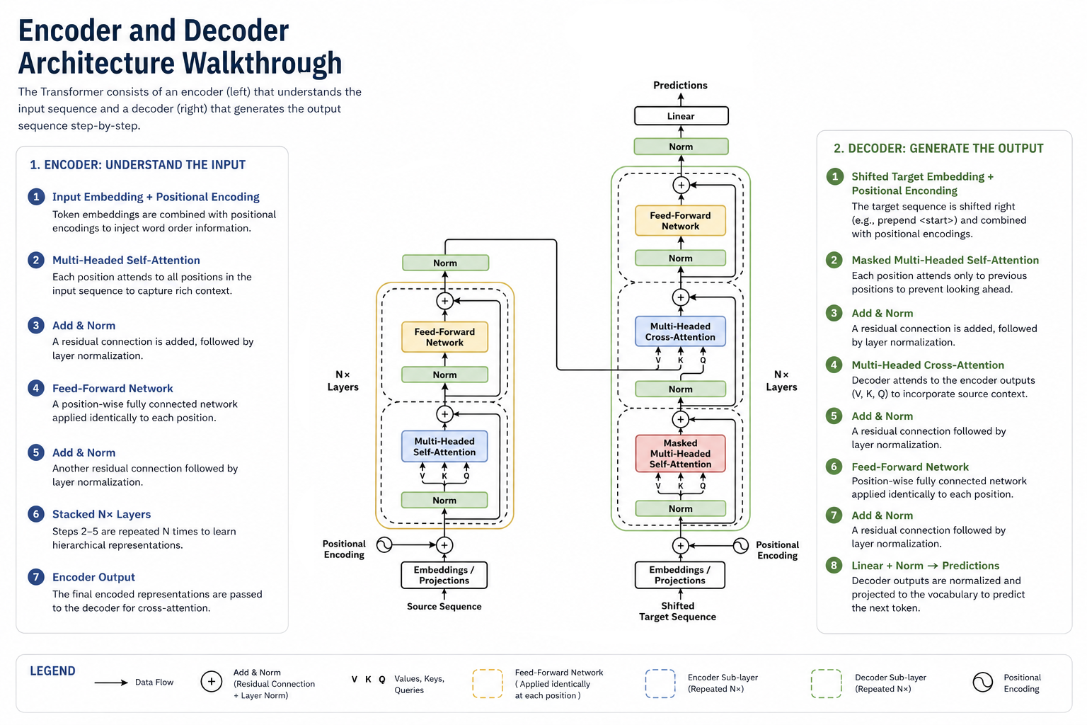
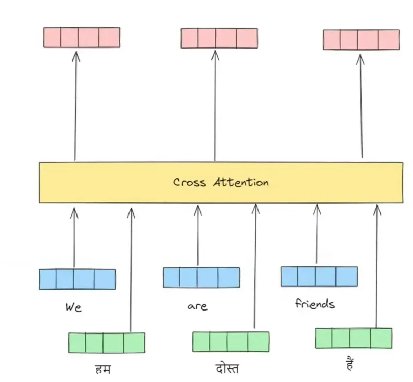
Transformers are encoder-decoder sequence transduction models. The Encoder takes a source sentence (English) and the Decoder generates a target sentence (Spanish) token-by-token.
GoalAccept source input and prepare the sequence translation context.
AnalogyLike having a book in English on the left table, and a notebook on the right table where you will write the translation page-by-page.
Source Sequence (Encoder Input)
Attention is all you need
Target Sequence Prefix (Decoder Input)
<bos> La atención es todo lo que
💡 Next Step target word: The model will predict the next word in the Spanish translation (which should be "necesitas").
Step 2 — Byte-Pair Encoding (BPE) Tokenization
Computers cannot read text directly. A tokenizer splits text into sub-words (tokens) and converts them into indices from a pre-defined Vocabulary list (V = 37,000 words/symbols).
GoalBreak raw text into standard numerical pieces (vocabulary IDs).
AnalogyLike looking up words in a dictionary index to convert a sentence into a series of page numbers.
Source Tokens & Vocabulary IDs (Click any token to inspect details)
Token Inspector
Click a token above to inspect character indexes and statistics.
⚙️ BPE Algorithm: It iteratively merges the most frequent pairs of characters/bytes. This prevents "Out-of-Vocabulary" errors by breaking unknown words down into smaller subwords (like "transformer" → ["trans", "former"]).
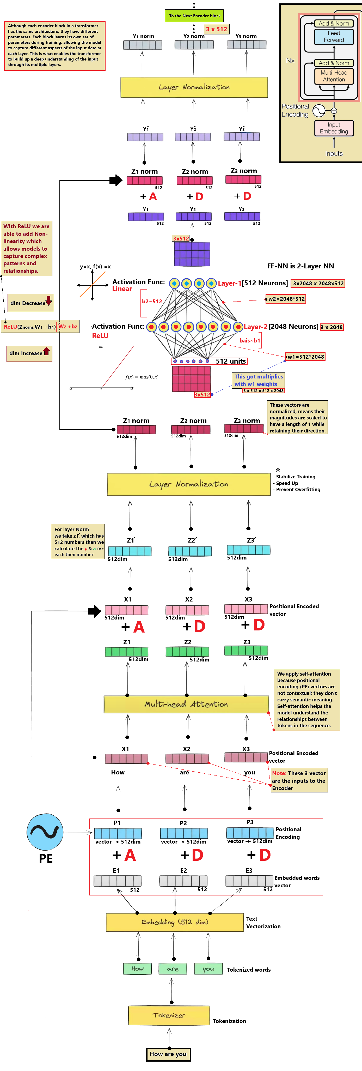
Step 3 — Token Embedding Lookup (d_model = 512)
Each Token ID is used to lookup a 512-dimensional vector. These vectors represent the semantic meaning of the token in a continuous vector space where similar concepts cluster together.
GoalTranslate discrete word indexes into semantic vectors representing meaning.
AnalogyLike looking up GPS coordinates on a multi-dimensional map where related words are located close to each other.
Embedding Matrix Grid (Hover cells to view specific dimensions)
Hover over cells to see float values and dimension numbers.
📊 Shape: `[Sequence Length × 512]`. Each row is a 512-element vector containing floating-point numbers learned during training.
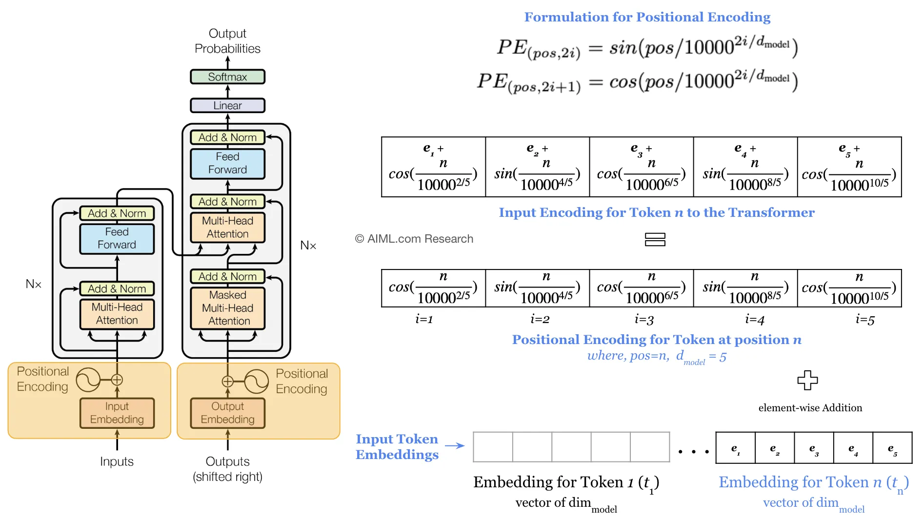
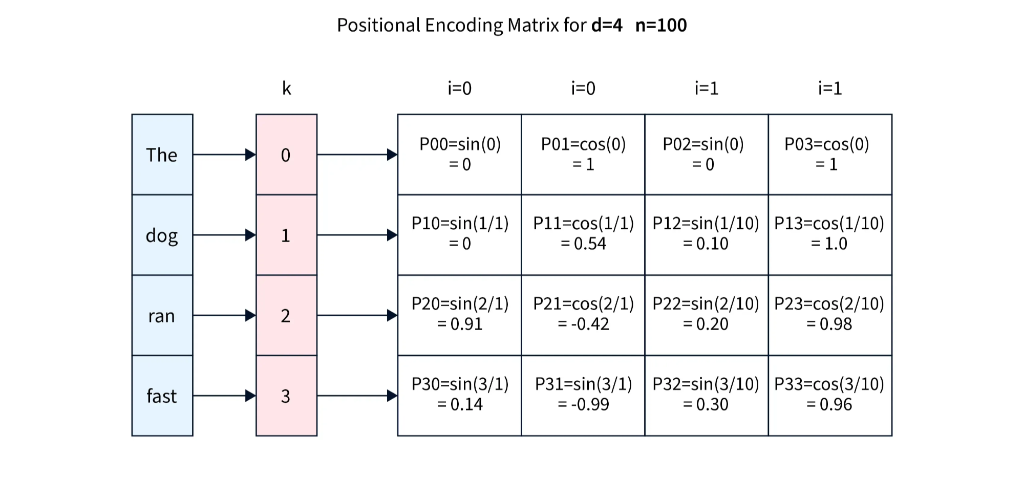
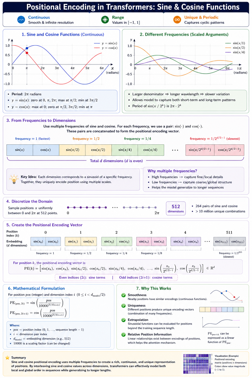
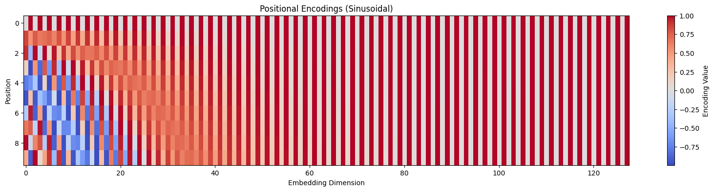
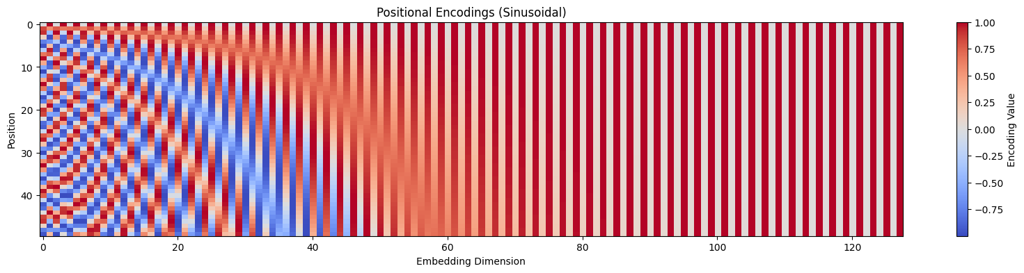
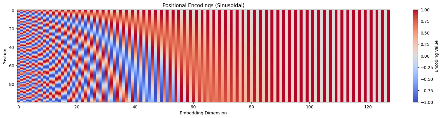
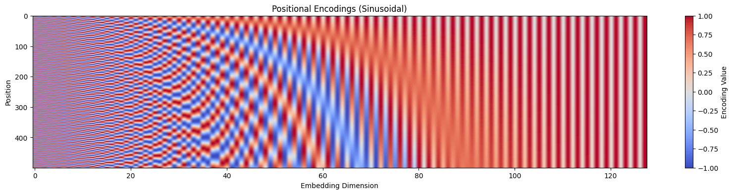
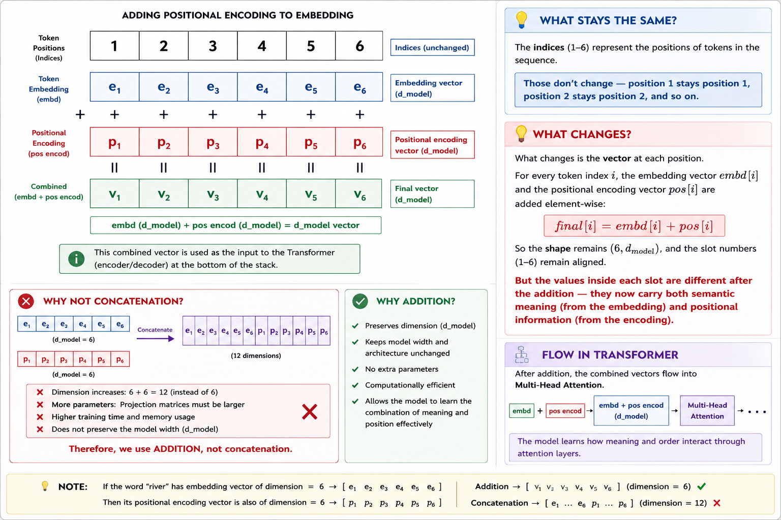
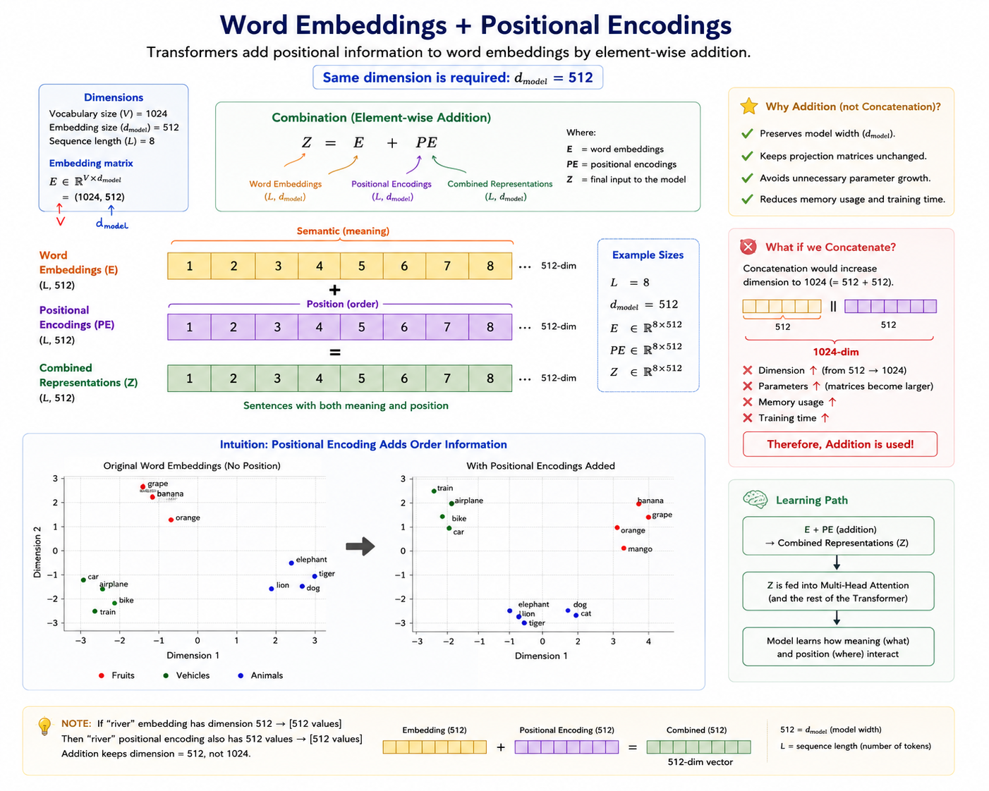
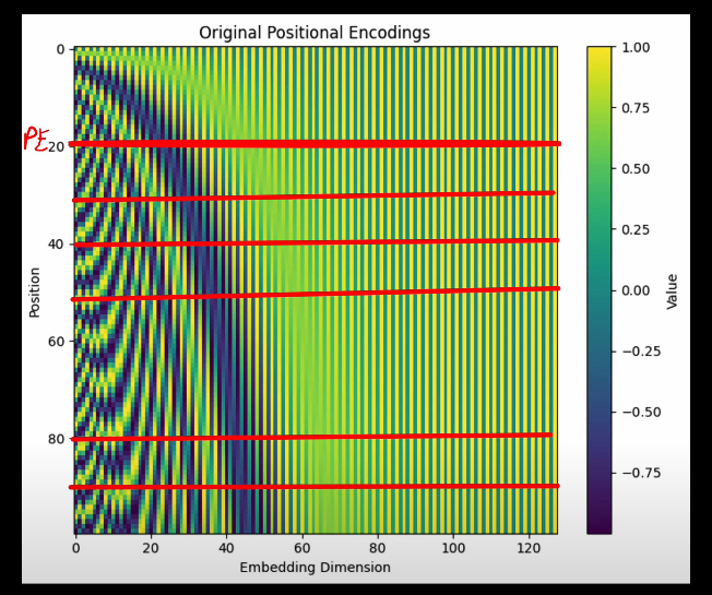
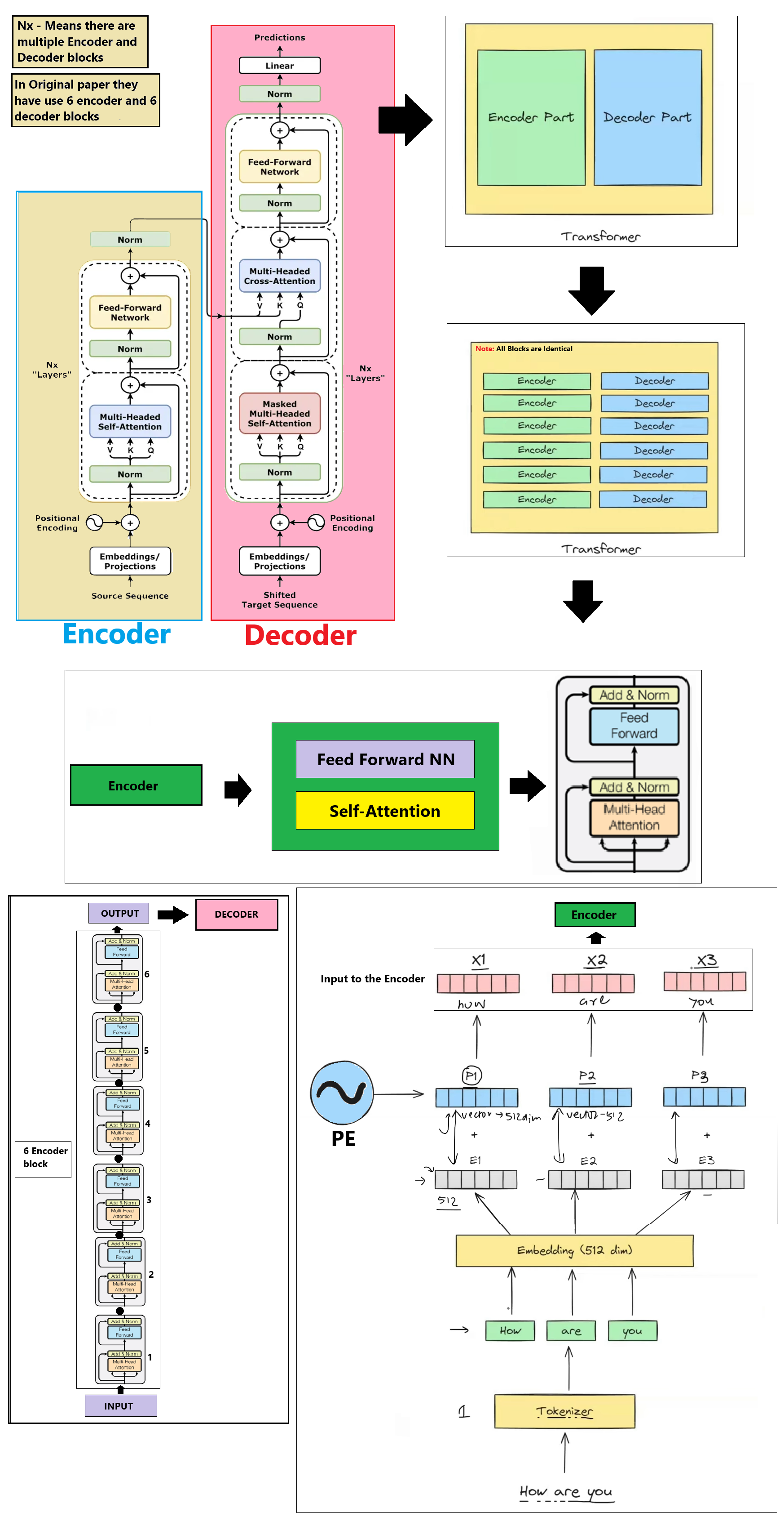
Step 4 — Sinusoidal Positional Encoding Injection
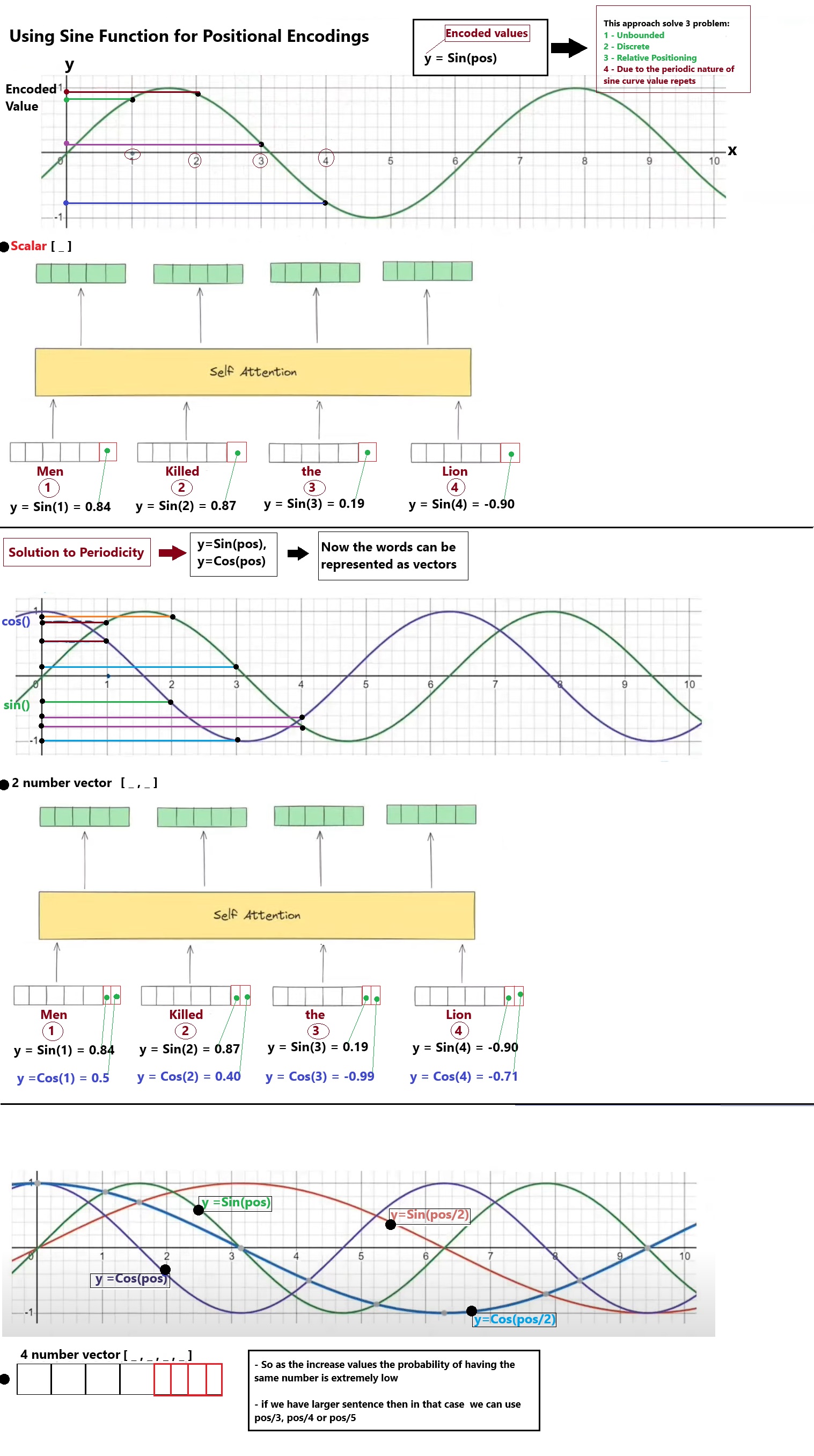
Self-attention processes all words in parallel, losing order information. To fix this, fixed sine/cosine waves of different frequencies are added element-wise to the embeddings.
GoalInject word position information without using sequential recurrences.
AnalogyLike writing a date watermark on letters so that even if they are delivered out of order, you can easily sort them.
Sinwave (Even Dim)
Coswave (Odd Dim)
1
0
PE(pos=1, dim=0) = sin(...) = ...
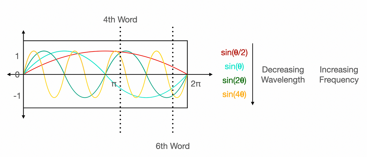
🧮 Formula:PE(pos, 2i) = sin(pos/10000^(2i/d)) PE(pos, 2i+1) = cos(pos/10000^(2i/d)). This enables the model to extrapolate to longer sequences than seen during training.
The Encoder uses a stack of 6 identical layers. In each layer, tokens attend to each other via Self-Attention to gather contextual information, then pass through a Feed-Forward Network.
GoalUnderstand each word in context (e.g. linking "bank" to "river" or "money").
AnalogyLike a group meeting where every person (word) makes eye contact (attention) with all others to establish relationships.
Encoder Layer 1 (Active)Interactive Node Graph
Attention Head:
Self-Attention Link Network (Hover/Click nodes to check links)
Encoder Layers 2–6Stacked
1. Dimension Flow Map
Follow how the shapes transition. Hover over a box to learn about its dimensions.
$Z$$[T \times 512]$
➔
$Q, K, V$$[T \times 64]$
➔
$Q K^T$$[T \times T]$
➔
$\text{Attention} \cdot V$$[T \times 64]$
Hover over any shape above to inspect its details.
2. Interactive Matrix Multiplier Sandbox
Choose a step to explore how rows and columns multiply. Hover over cells in the output matrix (C) to see the dot product animation.
Z$[T \times 512]$
×
W_Q$[512 \times 64]$
=
Q$[T \times 64]$
Hover over an element in the output matrix to trace its dot product calculation.
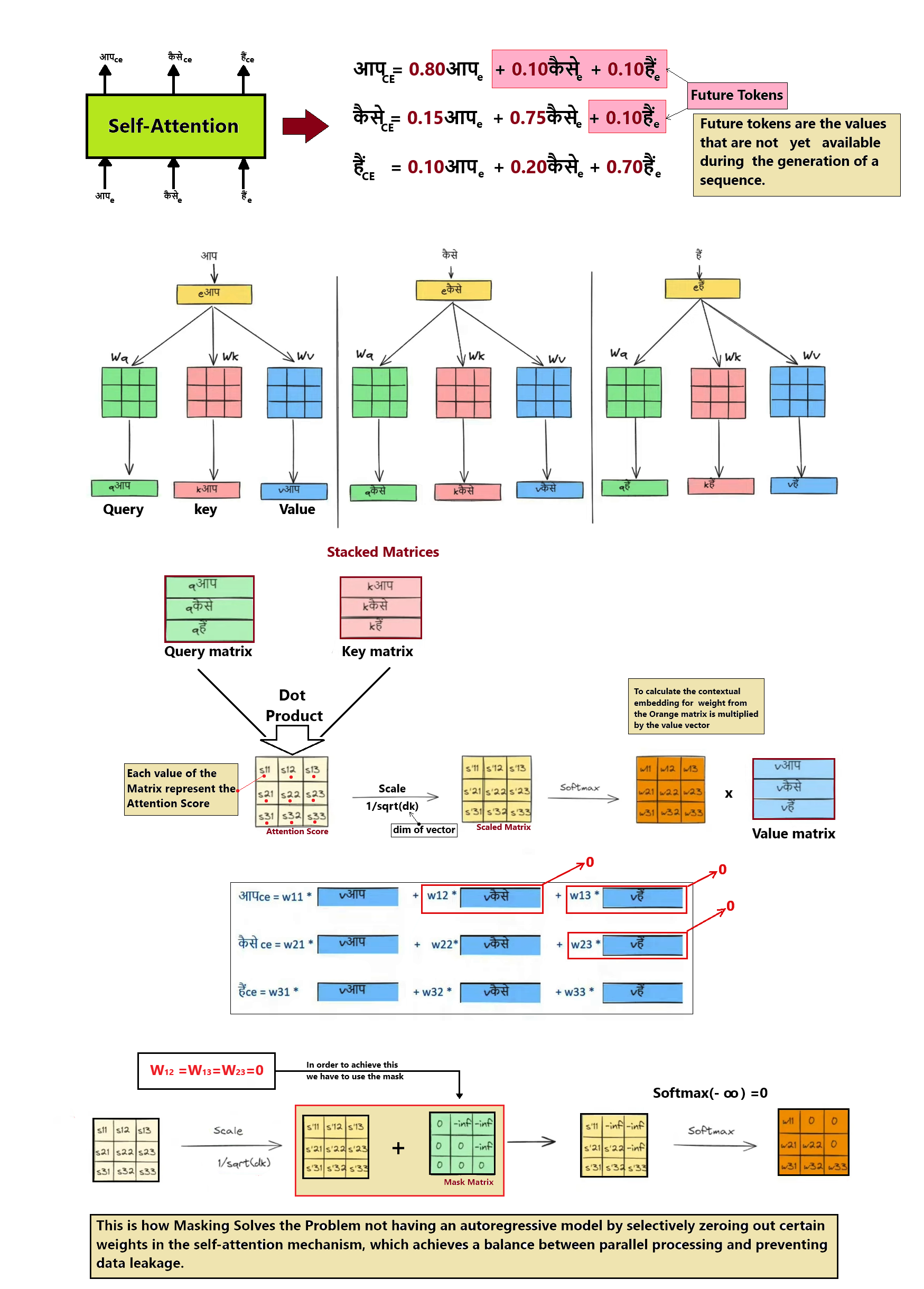
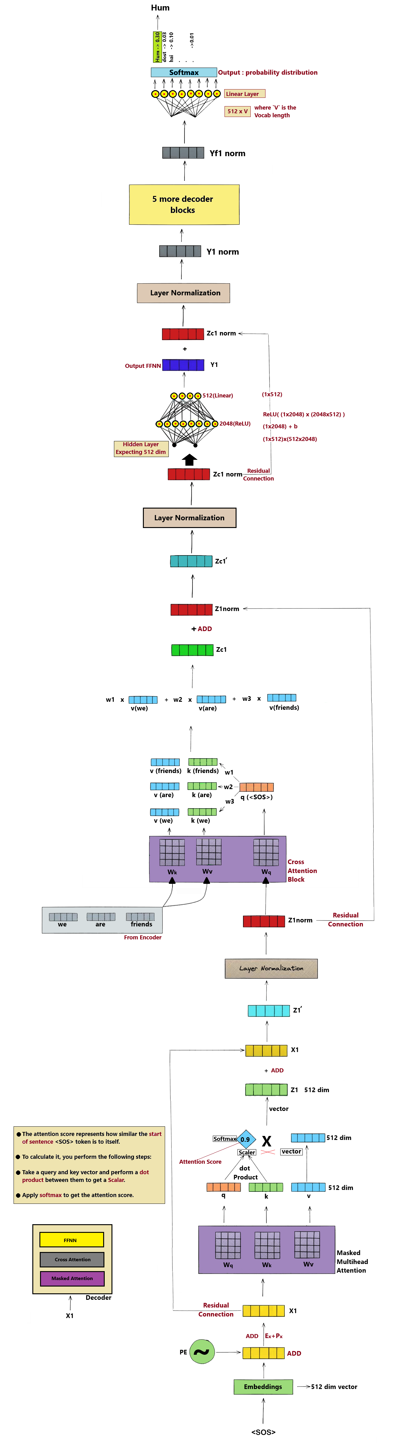
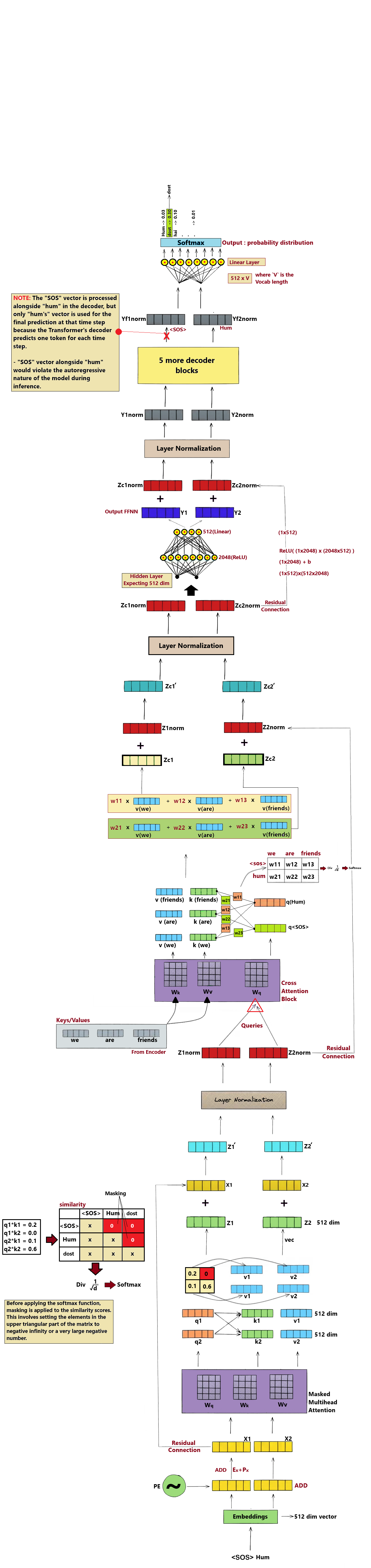
Step 6 — Decoder Layer Stack & Attention Masking
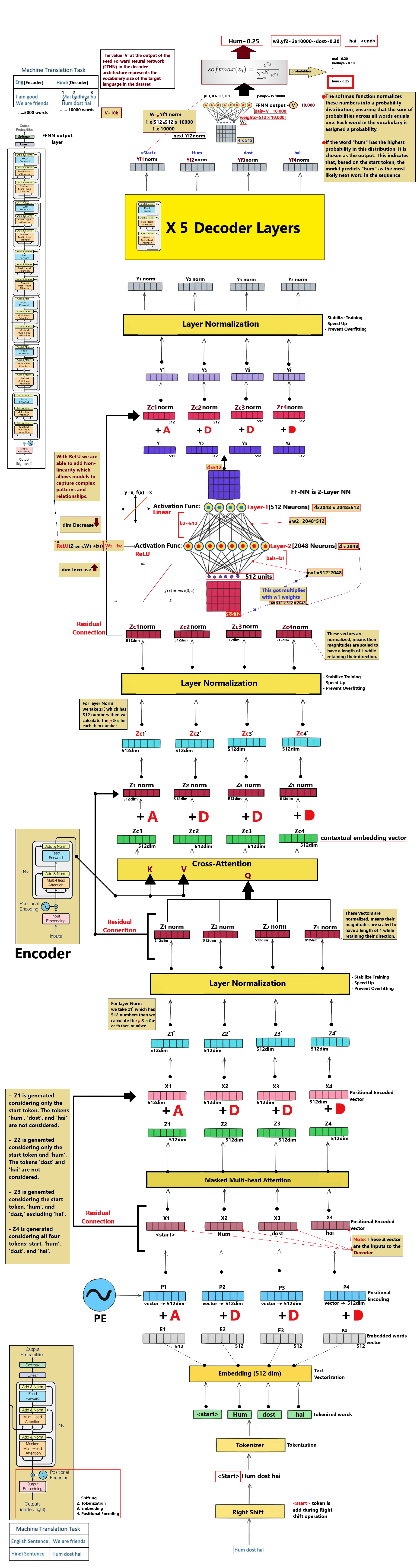
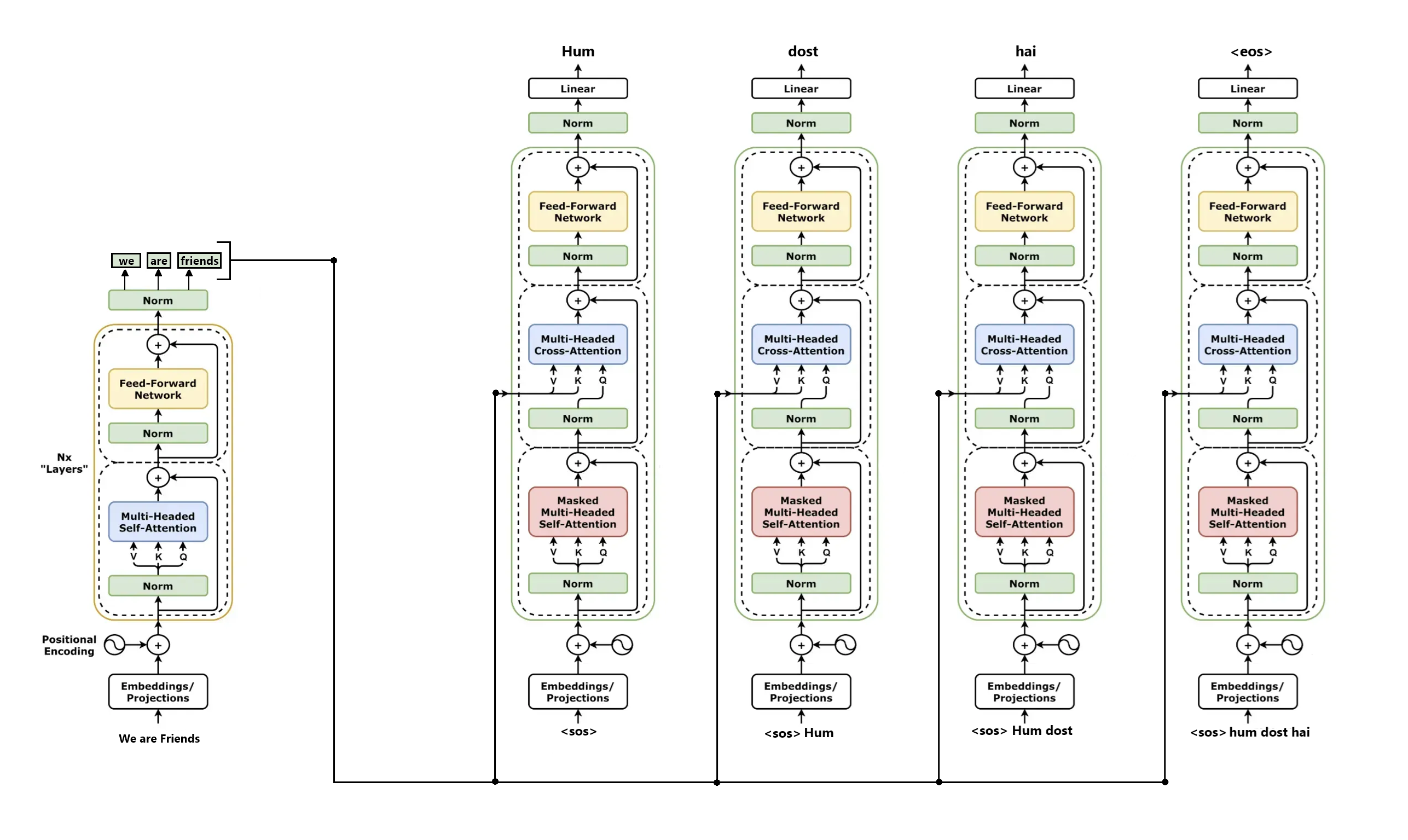
The Decoder stacks 6 layers to generate target tokens. It first applies Masked Self-Attention (protecting future tokens), then performs Cross-Attention to read Encoder outputs.
GoalGenerate translation step-by-step while attending to source memory and preventing looking ahead.
AnalogyLike translating a sentence where you are blindfolded to future parts of the sheet but have a clear look at the English original.
The output of the final Decoder layer is a 512-dim vector for the active position. The Linear layer projects this back to the size of our Vocabulary (37,000 logits).
GoalExpand low-dimensional representation to match the word options count.
AnalogyLike projecting a slide onto a giant wall of vocabulary tiles to highlight which tile matches the slide.
Decoder Output
[1 × 512]
×
Projection Matrix W
[512 × 37,000]
=
Output Logits
[1 × 37,000]
📝 Logits: These are raw, unnormalized scoring values. A higher score means the model thinks that vocabulary index is more likely to be the correct next word.
Step 8 — Softmax Probabilities & Temperature Control
The Softmax function normalizes raw logits into a probability distribution. The values sum to 1.0 (100%), with each representing the probability of that word being the next token.
GoalConvert raw scores into positive percentages summing up to 100%.
AnalogyLike converting raw class votes into actual vote share percentages for every candidate.
The token with the highest probability is selected (greedy decoding) and printed. To generate the next word, the selected token is appended to the target prefix, and the loop restarts.
GoalEmit the final word and feed it back to start generating the next one.
AnalogyLike translating a sentence word-by-word, where each word you write down helps you figure out the sentence flow.
...
→Appended to Target Sequence
New Decoder Input
→
<bos>...
🔄 Auto-Regressive translation: The model generates translation tokens one-by-one. Generation stops when the model outputs the special end-of-sequence token <eos>.
Recommended order
Study Path
Read in this order if you want the architecture to feel connected instead of scattered.
3. Full ArchitectureFollow the encoder stack first,
then the decoder stack with masking, cross-attention, and autoregressive output
generation.
Part 1 · Foundation
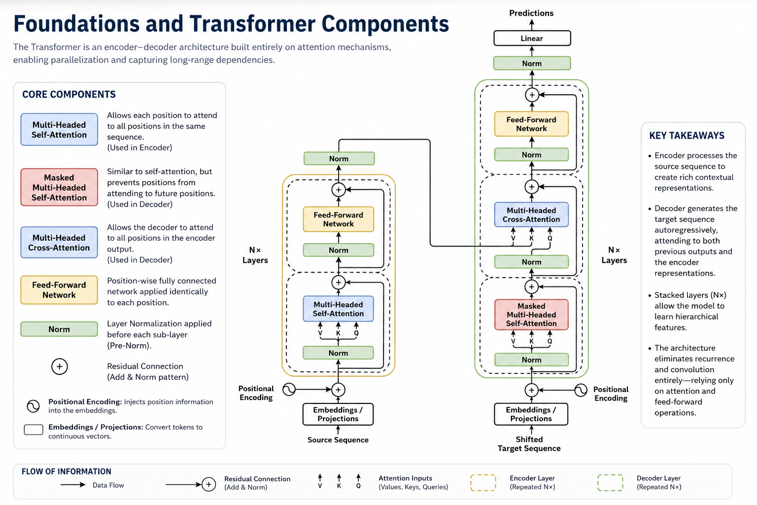
Foundations and Transformer Components
This part introduces the Transformer idea, the NLP timeline, attention, embeddings, positional
encoding, multi-head attention, residual connections, feed-forward networks, and normalization.
01 - Introduction to Transformers
⭐ Overview
🔴 The Paradigm Shift: The Transformer architecture, introduced in late 2017, abandoned sequential recurrence (RNNs/LSTMs) entirely in favor of parallel self-attention.
🔴 Global Context: By processing all tokens simultaneously, it enables direct connection between any two words regardless of distance, solving the vanishing gradient and memory bottleneck issues.
🔴 Foundation of Generative AI: The Transformer serves as the universal backbone for modern Large Language Models (LLMs) like GPT, Claude, Gemini, as well as scientific breakthrough models like AlphaFold 2.
Transformer [Generates the dynamic contextual embeddings]
1. Core Concept & Sequence Tasks
Sequence-to-Sequence (Seq2Seq): Designed to transform one sequence (like text) into another. Typical sequence tasks include:
Machine Translation: Translating language (e.g., English to French) where order dictates meaning.
Text Summarization: Distilling a long document sequence into a short summary sequence.
Question Answering: Mapping context + question tokens to answer tokens.
Speech Recognition: Translating continuous audio waves into text sequences.
Simultaneous Processing: Unlike sequential models, Transformers ingest and process all tokens in a sequence at once, replacing step-by-step reading with matrix operations.
2. Historical Context & Paradigm Shift
Legacy Bottlenecks: Prior architectures (RNNs, LSTMs, GRUs) processed text sequentially:
Vanishing Gradients: Information was squashed or lost over long distances, making it hard to link distant words.
GPU Underutilization: Sequential steps prevent parallel processing, limiting models to small datasets.
"Attention Is All You Need" (2017): Google Brain researchers proposed discarding recurrence and convolutions entirely, utilizing **Self-Attention** to calculate dependencies globally and in parallel.
3. Key Components of the Architecture
The standard Transformer architecture consists of the following components:
Encoder: Reads the input sequence, processes relationships, and builds context-aware embeddings.
Decoder: Generates output tokens sequentially, attending to both previous outputs and Encoder representations.
Self-Attention: The engine that computes similarity weights between every pair of tokens.
Feed-Forward Network (FFN): Applies non-linear transformations individually at each position to capture complex facts.
Layer Normalization & Residuals: Stabilizes training and enables deep networks (skip connections) by preventing vanishing gradients.
4. Transfer Learning & AI Democratization
Pre-training vs. Fine-tuning:
Pre-training: Large-scale, self-supervised learning on massive internet datasets to learn grammar, facts, and reasoning (extremely expensive).
Fine-tuning: Adapting the pre-trained model to specific downstream tasks (e.g., classification, translation) with limited labeled datasets (cheap).
Democratization: Transfer learning allowed small groups and startups to build state-of-the-art tools using API services or fine-tuning open models (like LLaMA) without needing huge compute centers.
5. Scientific Frontiers & Multimodality
Beyond Text: Transformers have unified deep learning across vision (Vision Transformers / ViT), audio (Whisper), and biology (AlphaFold 2 for protein structure prediction).
Multi-Modality: A single Transformer architecture can now map multiple modalities (text, images, audio, video) into a shared vector space, enabling unified models like GPT-4o or Gemini.
6. Advantages & Disadvantages
Advantages: Parallel training, direct long-range dependencies, unified architecture, and excellent scaling capacity.
Disadvantages:
Quadratic Complexity: Attention scaling cost is \(O(N^2)\) with sequence length, making long context windows expensive.
Resource Intensive: High training cost, massive energy footprint, and hard-to-explain "black box" decisions.
7. Final Summary Table
Core Topic
Primary Mechanism & Key Idea
Paradigm Shift & Impact
Key Examples / Architectures
Transformer Architecture
Uses self-attention (no sequential processing) to weigh relationships between all tokens simultaneously.
Revolutionized AI by enabling fully parallelized training, replacing sequential bottlenecks of RNNs/LSTMs.
Original Transformer (2017), BERT (Encoder), GPT (Decoder)
Self-Attention
Each token dynamically calculates attention weights for every other token in the sequence.
Solves the long-term dependency problem; model understands context globally rather than locally.
Focus on efficiency (quantization, pruning), interpretability, and domain-expert models.
Moving towards specialized, optimized models that run locally, alongside massive multimodal generalists.
FlashAttention, MoE (Mixture of Experts), Edge AI
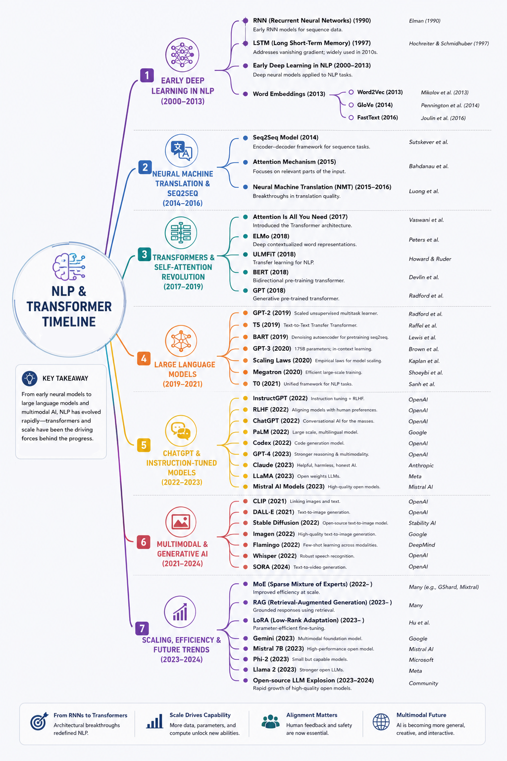
8. NLP Transformer Timeline
9. Practice Questions & Concept Intuitions
Q1: Why did the Transformer architecture represent a major paradigm shift in NLP?
Elimination of Sequential Bottleneck: Prior to the Transformer, state-of-the-art NLP models relied on recurrent neural networks (RNNs, LSTMs, GRUs) that read sequences word-by-word. The Transformer discarded this recurrence, using self-attention to process all tokens simultaneously, removing the sequential training bottleneck.
Massively Parallel Training: Because it processes all tokens at once rather than step-by-step, GPUs and TPUs can compute representations in parallel. This allowed models to scale to billions or trillions of parameters on massive datasets.
Overcoming Long-Range Constraints: In sequential models, information from early tokens fades over time during propagation. The Transformer creates direct paths between every word pair in a sequence, reducing the maximum path length between any two words to a constant \(O(1)\) operations regardless of sequence length.
Q2: What are the key limitations of sequential models like RNNs and LSTMs?
Strict Sequential Dependency: RNNs and LSTMs must compute hidden states step-by-step (calculating \(h_t\) only after \(h_{t-1}\) is done). This makes it mathematically impossible to parallelize training over the sequence length, leading to very slow training speeds on large corpora.
Vanishing and Exploding Gradients: Backpropagating errors through time requires repeatedly multiplying weight matrices. Over long sequences, this causes gradients to either decay exponentially (vanishing gradient, leading the model to forget early tokens) or grow exponentially (exploding gradient, leading to numerical instability).
Inability to Capture Global Context: Because sequence information is compressed into a single fixed-size hidden state vector at each step, details about long-range dependencies are lost, causing performance to degrade as sequences grow longer.
Q3: How do Transformers solve the vanishing and exploding gradient problems?
Direct Skip Connections via Self-Attention: The self-attention mechanism computes pairwise scores directly between any two tokens, regardless of distance. This keeps the path length between dependencies at \(O(1)\), meaning gradients do not have to flow through a sequence of steps to reach early inputs.
Residual Connections: Each sub-layer in a Transformer block is wrapped in a residual skip connection (e.g., \(x + \text{SubLayer}(x)\)). This forms a clean gradient highway during backpropagation, allowing gradients to flow directly to earlier layers without being altered by weight multiplication.
Layer Normalization: By normalizing activations across features at every layer, the model ensures that vector magnitudes remain in a stable numerical range, preventing exploding gradients and enabling the use of higher learning rates.
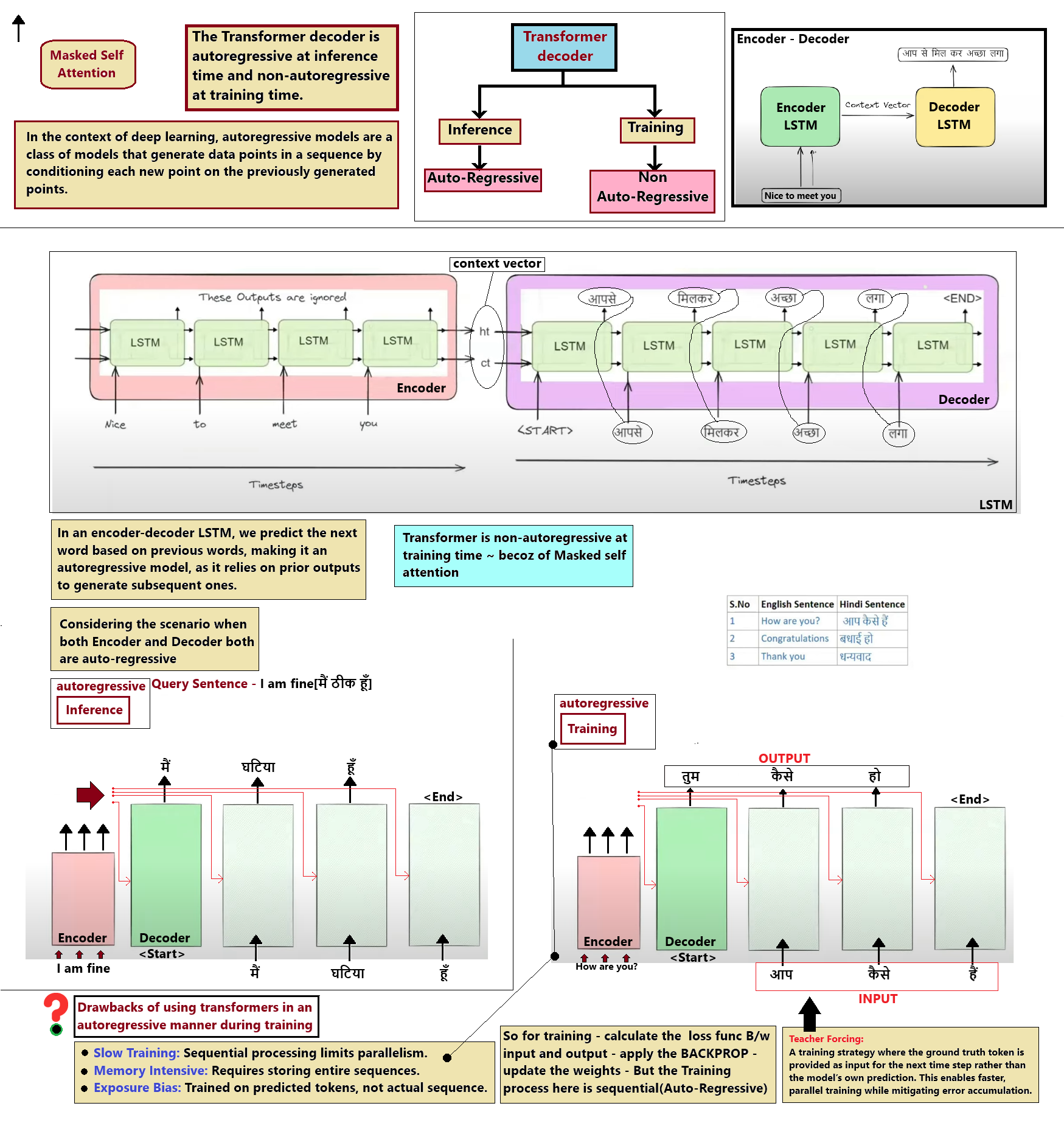
Q4: What is the difference between autoregressive and autoencoding Transformer architectures?
Autoregressive (Decoder-only): These models generate text token-by-token from left to right, where each generated token is appended to the input for the next step (e.g., GPT series). They utilize causal masking to prevent tokens from attending to future tokens, making them ideal for text generation.
Autoencoding (Encoder-only): These models receive the entire sequence at once and learn to reconstruct or denoise masked-out tokens (e.g., BERT). They utilize bidirectional self-attention, allowing every token to look at both past and future context, making them excellent for comprehension tasks like classification or question answering.
Sequence-to-Sequence (Encoder-Decoder): This hybrid setup combines both architectures, where the encoder processes the source sequence bidirectionally and the decoder generates the target sequence autoregressively (e.g., T5, BART). This is the standard framework for machine translation and summarization.
Q5: Why is transfer learning crucial for modern Transformer models?
Computational Feasibility: Pre-training a foundation Transformer model from scratch on large-scale datasets requires massive compute clusters and is cost-prohibitive. Transfer learning allows developers to download pre-trained weights and fine-tune them using single-GPU setups.
Data Efficiency: Training a deep Transformer on a small, task-specific dataset leads to severe overfitting. A model pre-trained on billions of words already understands syntax, grammar, and world facts, requiring very few labeled examples to adapt to a new task.
Emergent Generalization: Pre-trained models capture generalizable representations that perform well across multiple downstream tasks (zero-shot or few-shot learning), meaning a single pre-trained model can be adapted to hundreds of diverse applications.
Q6: How does pre-training differ from fine-tuning in the Transformer pipeline?
Pre-training Phase: The model is trained on a massive, unlabeled text corpus using self-supervised objectives, such as predicting a masked word (masked language modeling) or predicting the next token (causal language modeling). This phase builds the model's foundational linguistic and semantic capabilities.
Fine-tuning Phase: The pre-trained model is trained on a smaller, labeled dataset using a supervised objective, such as mapping a document to a sentiment class. The weights are gently adjusted to specialize the model for this target task.
Scale and Hyperparameters: Pre-training uses large batch sizes, high learning rates, and runs for weeks or months. Fine-tuning uses very small learning rates (to avoid destroying pre-trained knowledge), small batch sizes, and converges in a few epochs.
Q7: What are the computational complexity differences between RNNs and Transformers?
Sequential vs Parallel Complexity: For sequence length \(N\) and hidden dimension \(d\), an RNN has a time complexity of \(O(N \cdot d^2)\) because it must perform sequential multiplications. A Transformer has an attention complexity of \(O(N^2 \cdot d)\) due to pairwise attention score calculations.
Sequence Length Scaling: When the sequence length \(N\) is smaller than the representation dimension \(d\) (which is common, e.g., \(N=512, d=1024\)), Transformers are computationally highly efficient. However, for extremely long sequences (e.g., \(N > 32k\)), the quadratic \(O(N^2)\) scaling dominates memory and FLOP requirements.
Parallelizability: RNN operations are sequential and cannot be split across time steps on a GPU, whereas Transformers perform all pairwise attention dot products in parallel, allowing near-optimal GPU utilization.
Q8: Explain the contribution of the paper "Attention Is All You Need".
Rejection of Recurrent Architectures: The paper demonstrated that recurrent and convolutional structures are completely unnecessary for sequence transduction tasks, replacing them with a purely attention-based architecture.
State-of-the-Art Machine Translation: It achieved record BLEU scores on English-to-German and English-to-French translation tasks while training in a fraction of the time required by recurrent models.
Establishment of the Modern Transformer: It defined the core blocks used in NLP today: sinusoidal positional encodings, scaled dot-product attention, multi-head attention, residual blocks, and layer normalization.
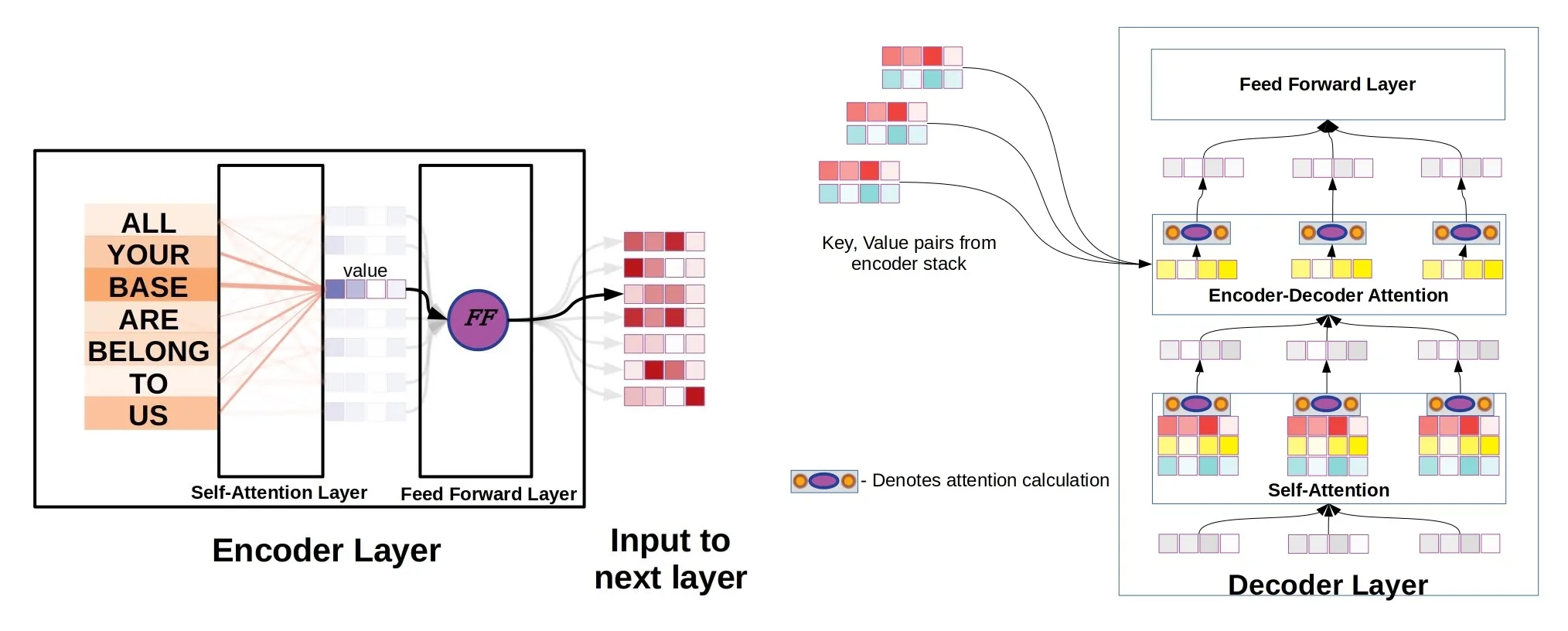
Q9: What roles do the Encoder and Decoder play in seq-to-seq tasks?
Encoder's Contextualization: The encoder processes the full source sequence bidirectionally, generating a continuous representation. Each token in the source sequence can attend to all other tokens, capturing structural and semantic context.
Decoder's Autoregressive Generation: The decoder generates the output sequence step-by-step. It uses causal self-attention to prevent looking ahead at future tokens, ensuring it only relies on tokens generated so far.
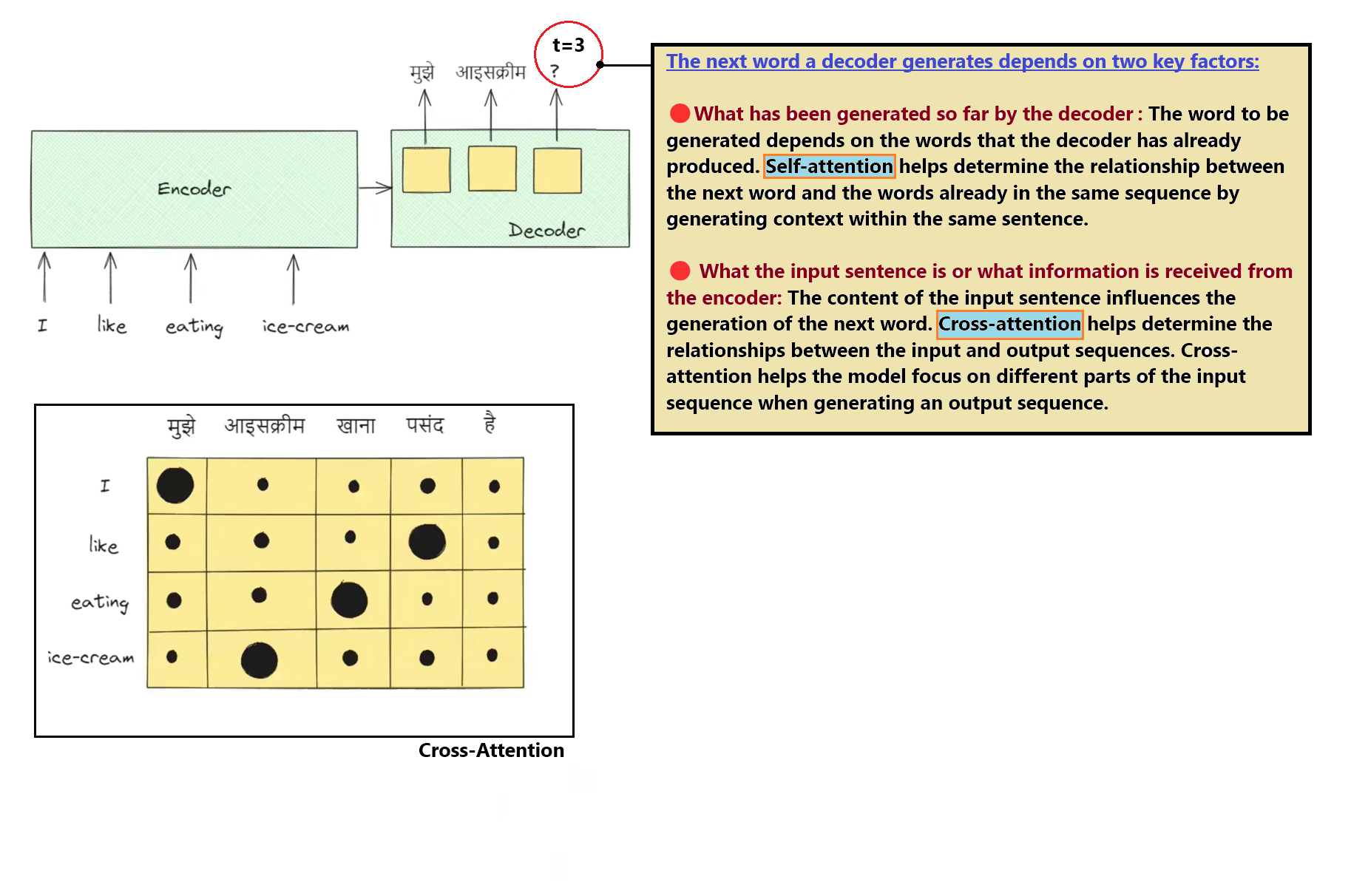
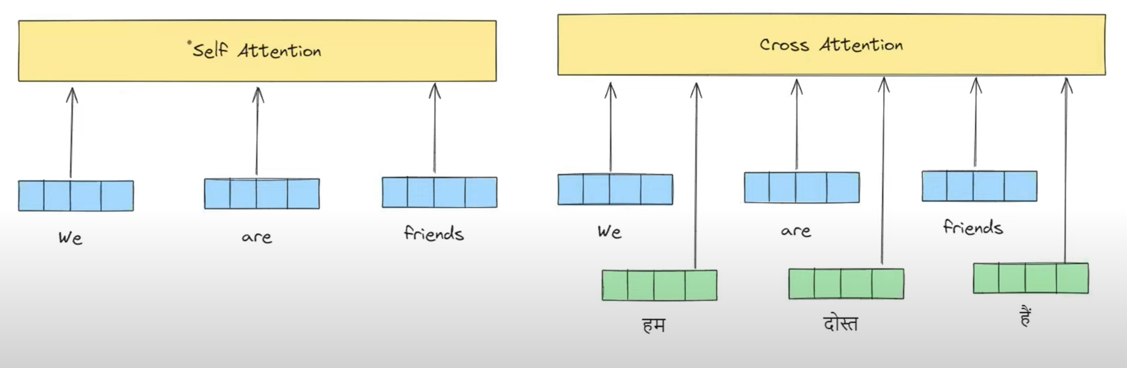
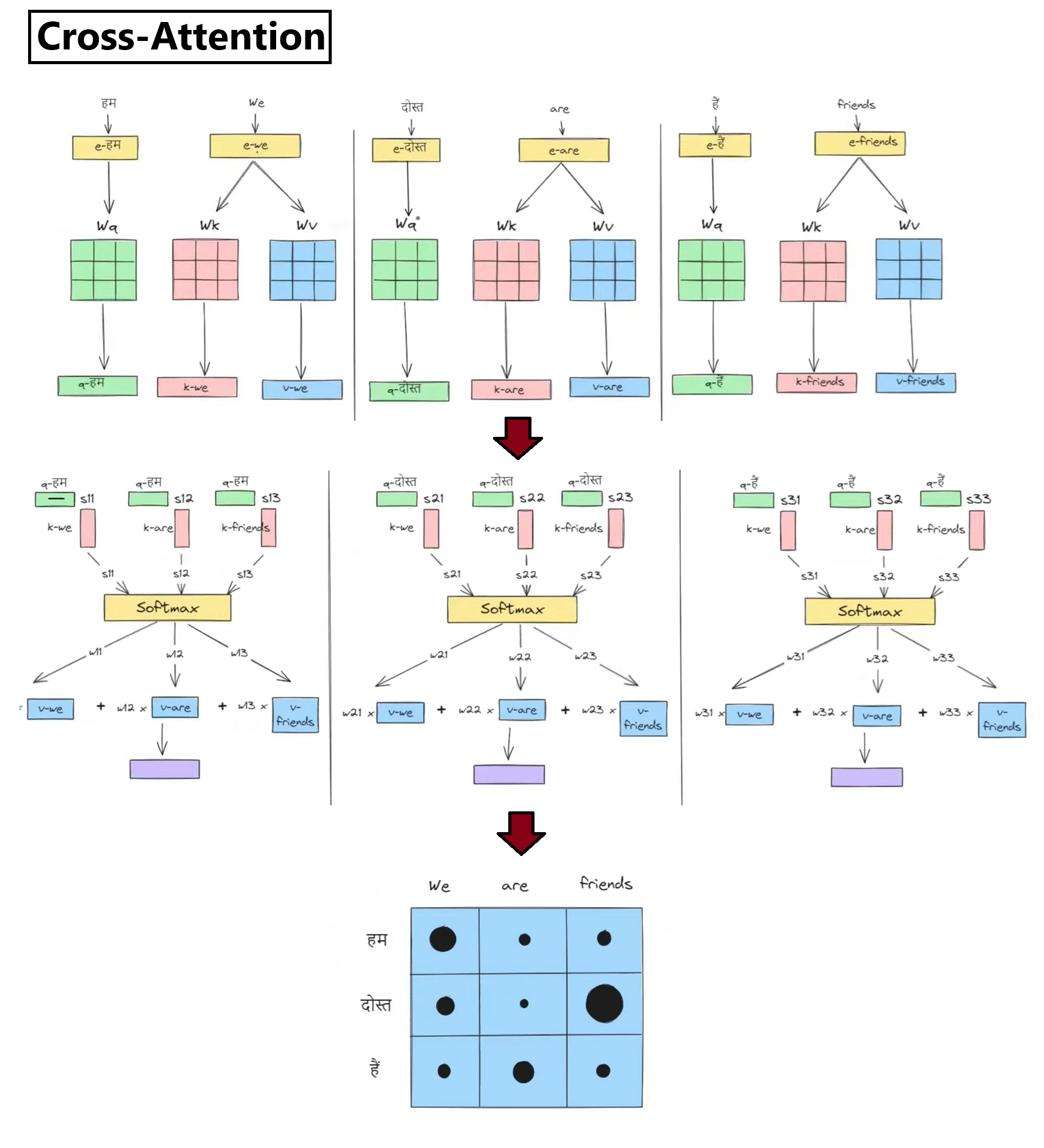
Cross-Attention Interface: The decoder connects to the encoder using cross-attention layers. Here, queries are projected from the decoder's state, while keys and values are projected from the encoder's output. This allows the decoder to selectively fetch relevant information from the source sequence during generation.
Q10: What is a key-value memory representation in the context of Feed-Forward networks?
Detecting Patterns (Keys): The first linear layer in the FFN projects the token embedding to a higher dimension (typically \(4 \times d_{\text{model}}\)) using a non-linear activation (like ReLU or GELU). Geometrically, this acts as a database lookup where the layer detects specific combinations of input features (keys).
Updating Representations (Values): The second linear layer projects the activated representations back to the original dimension. This layer outputs adjustment values that are added to the token's embedding, updating its semantic information based on the detected features.
Complementing Self-Attention: While self-attention moves information *between* tokens to establish relational context, the FFN operates on each token *individually*, acting as a static memory store that encodes factual and linguistic knowledge.
Q11: What is the unified framework concept in deep learning brought by Transformers?
Single Backbone Architecture: Before the Transformer, different domains used entirely different neural network templates (CNNs for computer vision, RNNs for speech and text, DSP for audio). The Transformer has unified these fields, serving as the standard model architecture across modalities.
Homogeneous Tokenization: All data formats are converted into a flat sequence of token embeddings: text words, image patches (Vision Transformers), audio spectrogram segments, or protein amino acids. Once tokenized, they are processed by the exact same self-attention layers.
Multi-modal Alignment: This structural homogeneity makes it easy to train models that process multiple modalities simultaneously (e.g., GPT-4o, Gemini), projecting text, images, and audio into a shared semantic space where they can interact directly.
Q12: How does AlphaFold 2 leverage Transformer architectures for protein folding?
Representing Amino Acid Sequences: AlphaFold tokenizes the primary structure of amino acid chains, treating residues like words in a sentence and searching database templates to align multiple sequences.
Evolutionary and Spatial Attention: It uses an attention block (Evoformer) to reason about co-evolutionary patterns and spatial relationships. The attention maps learn which amino acids must fold close together in 3D physical space, even if they are far apart in the linear chain.
Direct Geometric Output: The attention layers refine pairwise distance matrices, which are then projected into 3D coordinates, successfully predicting protein structure at atomic resolution.
Q13: What are the main disadvantages or computational challenges of Transformers?
Quadratic Scaling Complexity: Computing the self-attention matrix requires calculating compatibility between all token pairs, scaling as \(O(N^2)\) in memory and time. This makes processing extremely long documents, high-resolution images, or long audio files very resource-intensive.
Inference Bottleneck (KV Cache): During autoregressive generation, the model must store keys and values of all previous tokens (the KV cache) to avoid recomputing them. This cache scales with batch size and context length, bottlenecking GPU memory and throughput.
High Training Barrier: Training state-of-the-art foundation models requires thousands of GPUs running for months, which has a significant carbon footprint and limits development to well-funded organizations.
Q14: What is the impact of model scaling (laws of scaling) on Transformer performance?
Predictable Power-law Performance: Research shows that loss scales as a power-law relationship with the number of model parameters, training tokens, and training compute. This allows researchers to predict model performance before investing in massive training runs.
Emergent Capabilities: As models scale past certain thresholds (e.g., billions of parameters), they exhibit sudden, qualitatively new capabilities (such as multi-step reasoning, coding, and translation) that were completely absent in smaller configurations.
Parameter vs. Token Trade-offs: Scaling laws show that for optimal performance, model size and dataset size must scale in equal proportions (compute-optimal training, as demonstrated by the Chinchilla scaling laws).
Q15: What are multi-modal Transformers, and how do they integrate different data modalities?
Cross-modality Tokenization: Non-textual inputs are converted into standard token sequences. For example, an image is split into \(16 \times 16\) patches, projected into linear embeddings, and prepended or appended to the text tokens.
Joint Attention Routing: Once tokenized, all inputs are processed by standard multi-head self-attention. The model computes attention scores across textual and visual tokens, allowing the representation of a text token to directly incorporate visual features (and vice versa).
Unified Cross-Attention: Alternatively, a text-based decoder can use cross-attention to attend to features generated by a separate vision encoder (e.g., Flamingo model), aligning the representation of different data streams.
02 - What is Self Attention?
⭐ Overview
🔴 The Core NLP Problem: How do we represent human language as numbers in a way that captures meaning?
🔴 Static vs. Dynamic: Static embeddings (Word2Vec, GloVe) assign a single fixed vector to each word, failing to capture context (e.g., "apple" the fruit vs. "Apple" the company).
🔴 Self-Attention Breakthrough: Self-attention takes static embeddings and dynamically computes contextual embeddings based on neighboring tokens in the sequence.
1. The Fundamental NLP Problem
Numeric Translation: Computers process numbers, not raw text. NLP models require projecting words into a mathematical vector space (vectorization).
Contextual Ambiguity: Human language is highly contextual. A single word's meaning can change completely depending on the surrounding tokens (homonyms and polysemy).
2. Evolution of Word Vectorization Techniques
Before modern deep learning, three primary vectorization methods were used to represent text:
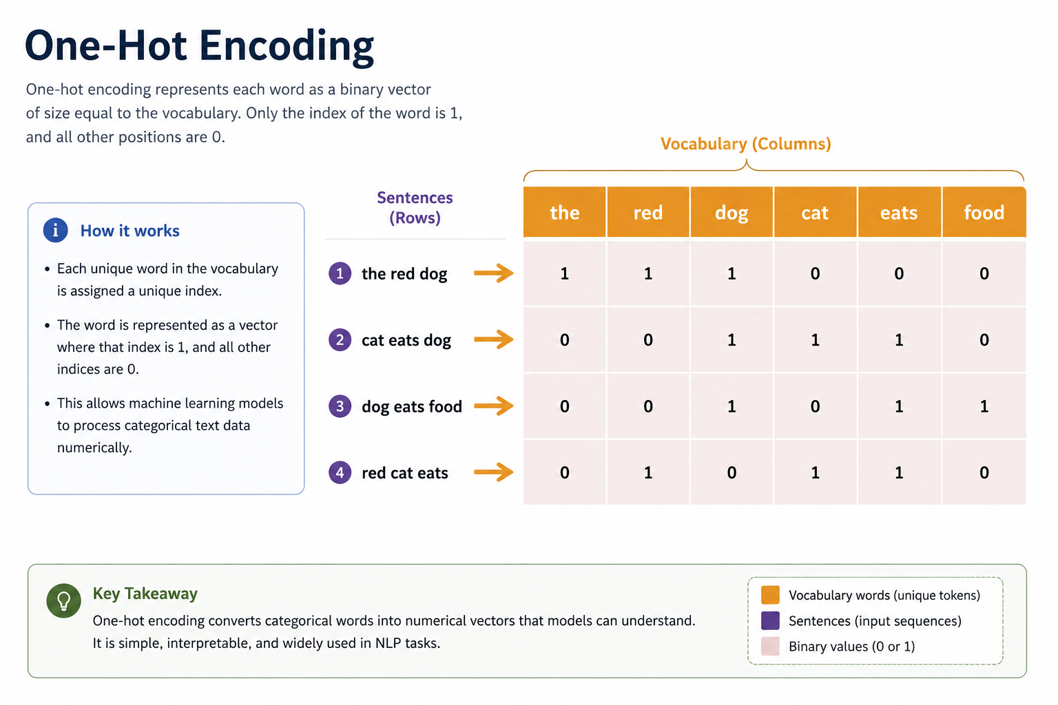
One-Hot Encoding
Mechanism: Maps each unique word to a sparse binary vector whose size equals the vocabulary size, containing a single 1 at the word's index.
Limitations: High-dimensional, extremely sparse (mostly zeros), and captures zero semantic similarity or relationships between words.
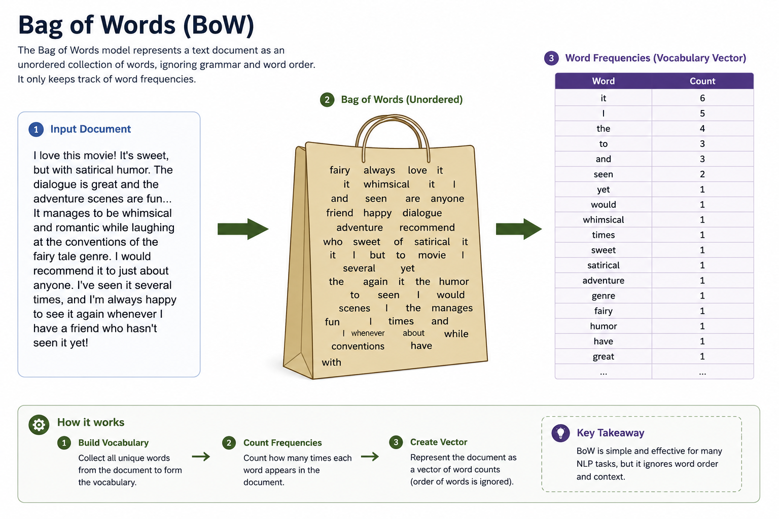
Bag of Words (BoW)
Mechanism: Counts occurrences of each word in a document or sentence.
Limitations: Discards word order, grammar rules, context, and semantic similarity.
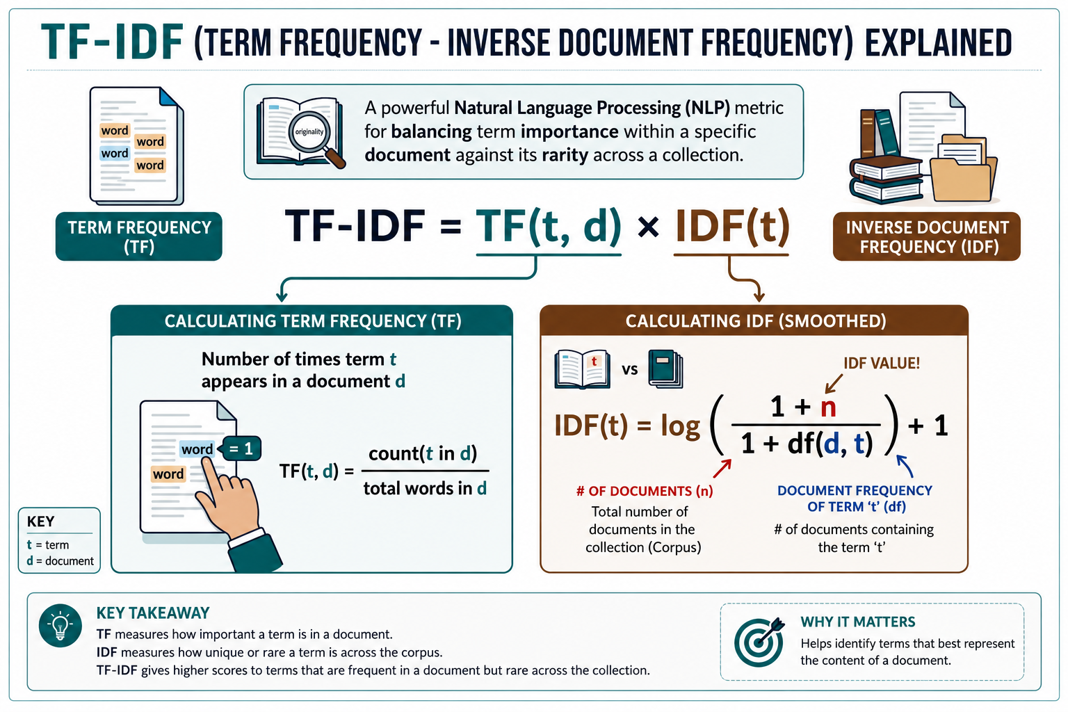
Mechanism: Weights words by multiplying term frequency (local occurrence) by inverse document frequency (global rarity).
Limitations: Excellent for search and retrieval, but still treats words as isolated entities without contextual understanding.
3. Static Word Embeddings & Their Limits
Dense Vectors: Static embeddings (e.g., Word2Vec, GloVe) map words to low-dimensional, continuous dense vectors (e.g., 300 dimensions).
Semantic Proximity: Words with similar meanings sit close together in geometric space (e.g., the vectors for king and queen are close).
The Static Constraint: A word always receives the same fixed vector representation, regardless of context. For example:
In "Apple launched a new phone" and "I ate a green apple", the vector for apple is identical, resulting in an "average" meaning that mixes technology and fruit.
4. Self-Attention: Dynamic Contextual Embeddings
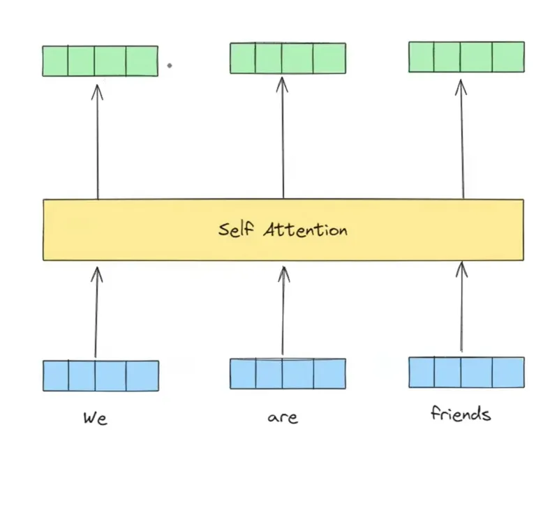
Dynamic Mapping: Self-attention solves the static constraint by generating **contextual embeddings** on the fly.
Interaction: Takes static embeddings for the entire sentence simultaneously, computes mutual dependencies, and outputs contextually adjusted vectors.
Ambiguity Resolution: In "Apple launched a new phone", self-attention maps the connection between Apple, launched, and phone to dynamically boost "technology" features and dampen "fruit" features of the Apple vector.
5. Real-World Applications of Self-Attention
Large Language Models (LLMs): Powers models like ChatGPT, Claude, and Gemini to generate coherent, context-rich text.
Machine Translation: Translates fluidly by resolving syntactic dependencies and homonyms.
Text Summarization & Sentiment Analysis: Accurately extracts key concepts and detects emotional tone by analyzing text globally.
Code Generation: Maps programming syntax and descriptions to construct working scripts.
Performs calculations using query, key, and value vectors to adjust static embeddings based on neighboring words in a sentence.
Generates dynamic embeddings that understand specific word contexts and resolve ambiguity.
Requires complex mathematical calculations.
Yes
Dynamic contextual embeddings
Transformers, Large Language Models (LLMs), Generative AI, Machine Translation
Word Embeddings (Static)
Neural networks trained on large datasets to convert words into n-dimensional vectors based on semantic similarity.
Captures semantic meaning; similar words occupy similar positions in geometric space.
Represents an "average meaning"; cannot distinguish between different meanings of the same word based on context.
No
n-dimensional dense vectors (e.g., 64, 256, 512)
Sentiment analysis, Named Entity Recognition (NER), general NLP tasks
TF-IDF
Weights the importance of words by multiplying Term Frequency by Inverse Document Frequency.
Improves upon Bag of Words by considering word importance across an entire document corpus.
Does not capture semantic meaning or contextual nuances.
No
Sparse vectors (weighted)
Document classification, information retrieval
Bag of Words (BoW)
Counts the frequency of each unique word within a specific document or sentence.
Captures word frequency, offering an improvement over binary one-hot representation.
Lacks semantic understanding and context; remains a relatively simple representation.
No
Sparse vectors (counts)
Simple NLP applications, sentiment analysis
One-Hot Encoding
Assigns a unique vector where one index is 1 and all others are 0 based on the presence of a word in a fixed vocabulary.
Simple and original method for converting words to numerical representations.
Inefficient for large vocabularies; creates high-dimensional, sparse vectors.
No
Sparse vectors (binary)
Basic vectorization in early NLP tasks
7. Practice Questions & Concept Intuitions
Q1: What is the fundamental NLP problem of word representations in varying contexts?
The Challenge of Polysemy: Many words have multiple meanings depending on context (e.g., "bank" the financial institution vs. "bank" of a river). A word's exact semantic value is not static; it is determined by the words that surround it.
Static representation limits: Traditional representation models (like Word2Vec or GloVe) assign a single fixed vector to each word, which is the mathematical average of all its training contexts. These models cannot adapt the vector when a word is used in a specific sentence.
Contextual Disambiguation: Without dynamic adjustments, downstream neural network layers receive identical input vectors for different meanings, making it extremely difficult to parse sentence semantics accurately.
Q2: Explain how One-Hot Encoding works and why it fails to capture semantic meaning.
Sparsity Mechanism: Maps each vocabulary word to a vector of length \(V\) (vocabulary size) containing a single `1` at the word's index and `0`s elsewhere. For a vocabulary of 50,000 words, each word is represented by a 50,000-dimensional vector.
Orthogonal representations: Because every vector has a single `1` at a unique index, the dot product between any two distinct one-hot vectors is always exactly `0`. Geometrically, all word vectors are perpendicular (orthogonal) to one another, indicating that "cat" and "dog" are mathematically as unrelated as "cat" and "refrigerator."
Dimensionality Explosion: As the vocabulary grows, vector size scales linearly, leading to massive, sparse matrices that consume huge amounts of memory without holding any semantic relationships.
Q3: What is the Bag-of-Words (BoW) model, and what are its primary limitations?
Count Vectors: Represents a document as a histogram counting word occurrences, ignoring order and syntax structure. The document is mapped to a vector where each index represents the frequency of a vocabulary word.
Zero Context: Cannot capture grammar or relational meaning. The sentences "man eats fish" and "fish eats man" yield identical BoW representations because they share the exact same word counts, despite expressing opposite ideas.
Vocabulary Bias: Common words (like "the", "a", "is") dominate the representation because of their high frequency, while rare, topic-defining words get drowned out unless manually filtered.
Q4: How does TF-IDF improve upon Bag-of-Words representation?
Importance Weighting: Multiplies Term Frequency (TF - how often a word appears in a specific document) by Inverse Document Frequency (IDF - log of total documents divided by documents containing the word).
Dampening Common Words: If a word (like "the") appears in every document in a corpus, its IDF is \(\log(1) = 0\), completely neutralising its term weight. This highlights document-specific keywords (like "diabetic" or "quantum").
Static Limitations: Although it balances word importance across a corpus, TF-IDF remains a bag-of-words method. It does not model word order, grammar, or polysemy within a document.
Q5: What are static word embeddings (e.g., Word2Vec, GloVe), and what is their major limitation?
Dense Vector Projections: Project words into a low-dimensional dense space (typically 100-300 dimensions) where semantic similarity is captured by vector closeness (using cosine similarity). These representations are learned by predicting local context windows (Word2Vec) or global co-occurrence statistics (GloVe).
Static Mapping Limitation: Each word is assigned a single fixed vector. The vector representing the word "apple" is the same whether referring to the fruit, the tech company, or the record label, resulting in a blurred semantic average.
Out-of-Vocabulary (OOV) Issue: Static embeddings cannot generate representations for new or misspelled words unless subword tokenization (like FastText) is explicitly used.
Q6: How does self-attention generate dynamic, context-dependent word representations?
Pairwise Relationship Scoring: Self-attention calculates similarity scores between all tokens in a sentence. Every word is compared to all other words (including itself) to measure their semantic relevance.
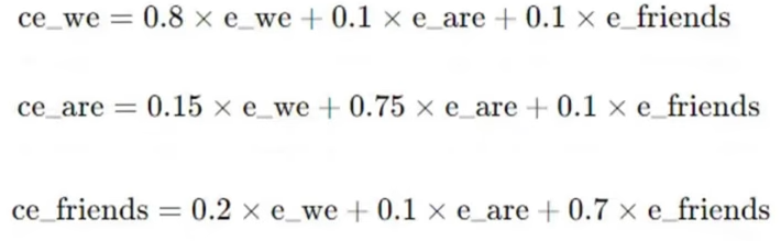
Dynamic Weighted Blending: The output vector for a token is computed as a weighted sum of all word embeddings in the sequence. If a word is highly relevant to the target token, its vector contributes more to the final representation.
Contextual Adaptation: By pooling information from its surroundings, the word's vector shifts its coordinates in the embedding space, dynamically adjusting its meaning to fit the sentence context.
Q7: What does "permutation invariance" mean in the context of self-attention?
Order-Agnostic Processing: Self-attention treats the input sequence as a set of tokens and does not have an inherent concept of order. If you shuffle the input sequence, the output vectors will shuffle but remain identical in values.
Commutativity of Dot Products: The similarity score between token \(i\) and token \(j\) depends purely on their vector values, not their position index.
Requirement for Position Encodings: To prevent the model from behaving as a simple bag-of-words, external positional encodings must be added to the input embeddings, injecting sequence order context.
Q8: Give a concrete example of how self-attention resolves polysemy (e.g., "bank").
River Context: In "The river bank is muddy," self-attention connects "bank" to "river" and "muddy," shifting its vector representation towards geographic dimensions.
Finance Context: In "The bank approved my loan," self-attention connects "bank" to "loan" and "approved," moving the vector representation towards financial coordinates.
Dynamic Coordinate Shifting: Rather than using a static, averaged vector, self-attention pulls features from surrounding keys, adjusting the coordinates of "bank" to reflect its specific meaning.
Q9: How does self-attention differ from sequential context processing in LSTMs?
LSTM Recurrence: Processes text step-by-step, carrying context in a hidden state. Context from earlier steps fades over long sequences.
Self-Attention: Direct pairwise calculations across the entire sequence. The distance between any two tokens is always 1, preventing information decay.
Parallel vs Sequential FLOPs: LSTMs must wait for prior hidden states to finish, while self-attention computes all token interactions in parallel, maximizing GPU performance.
Q10: What is the semantic relationship captured by the dot product of two word vectors?
Geometric Alignment: The dot product measures the projection alignment of two vectors. If they point in similar directions, the score is highly positive.
Semantic Mapping: High positive values indicate similar context or meaning alignment; values close to zero indicate orthogonal, unrelated concepts.
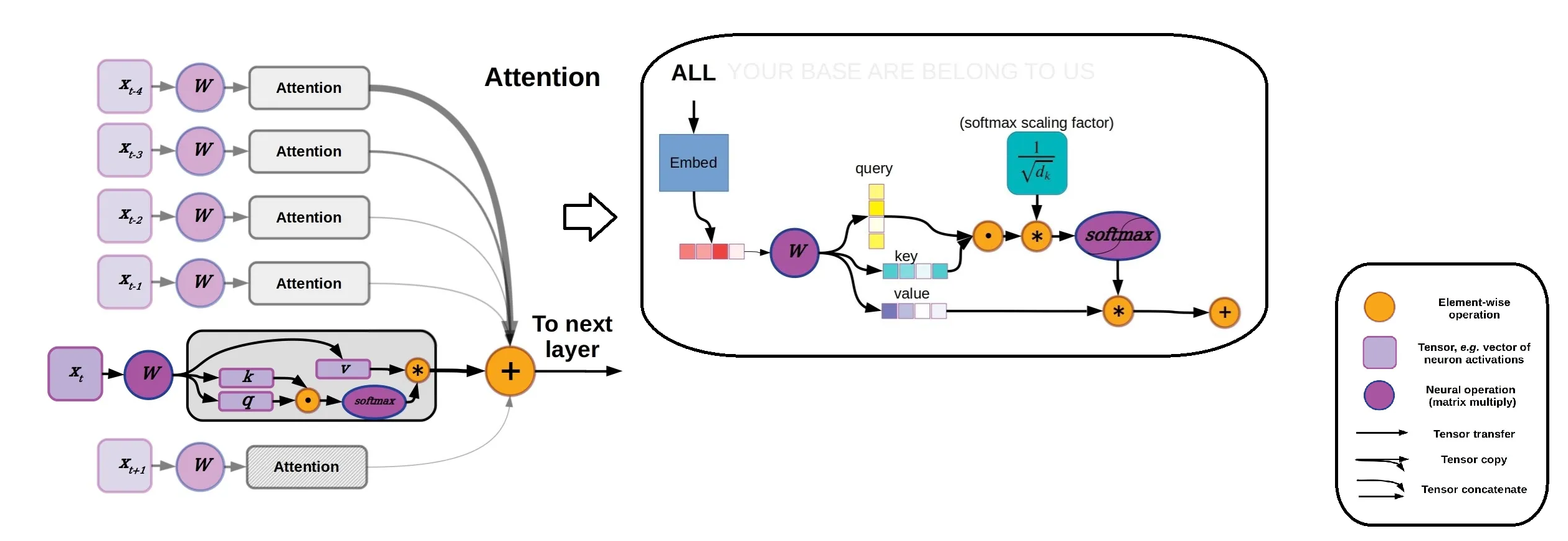
Magnitude Influence: The dot product scales with vector magnitudes. In self-attention, we divide by \(\sqrt{d_k}\) to prevent large dimensions from dominating similarity calculations.
Q11: How does self-attention compute the relevance of a token to all other tokens in a sequence?
Attention Coefficients: Takes query-key dot products for all pairs, scales them, and applies Softmax.
Relative Weights: The resulting probabilities represent how much attention (or weight) each token should receive relative to the other words in the sentence.
Information Routing: These weights act as a filter, determining how much context is pulled from each token's value vector to construct the final representation.
Q12: Why is self-attention considered a "bag-of-words" model when positional signals are absent?
No Order Info: Because the dot product operation is commutative and independent of position index, the calculated scores depend purely on vector contents.
Identical Outputs: Shuffling word order would output the exact same set of updated embeddings, rendering the sequence representation order-invariant unless position indicators are added.
Geometric Permutation: Without positional coordinates, the Transformer treats the input sequence as an unordered set of tokens, losing grammatical structural context.
Q13: What are the real-world applications where contextual embeddings are highly critical?
Machine Translation: Where exact word translations depend on local gender, tense, or structural context.
Search Queries: Disambiguating search intent (e.g., searching for "jaguar speed" vs. "jaguar dealership").
Named Entity Recognition (NER): Identifying entities whose type depends on context (e.g., "Washington" as a person vs. a state).
Q14: How does the similarity scoring mechanism in self-attention enable global context modeling?
Parallel Connections: It calculates similarity weights for all token combinations simultaneously, allowing immediate long-range context association.
Context Aggregation: Rather than passing information through intermediate hidden states, words pool context globally in a single layer.
Syntactic Shortcuts: Direct pathways allow the model to link distant but related grammatical tokens (e.g., a subject and its verb at the end of a long clause).
Q15: How do word vectors "migrate" or change positions in the vector space after self-attention is applied?
Weighted Shift: The self-attention output is a weighted sum of value vectors. This shifts the original vector's coordinates in the high-dimensional space.
Contextual Realignment: Words in a shared context migrate closer together in space (e.g., "bank" moves closer to "river" dimensions), dynamically adjusting their semantic coordinates.
Feature Layering: As representations pass through multiple Transformer layers, their geometric coordinates continuously refine, moving from basic lexical markers to complex, context-rich semantic vectors.
03 - Self Attention in Transformers
⭐ Overview
🔴 Dynamic Transformation: Self-attention generates context-aware vectors on the fly, allowing each token's representation to evolve based on its neighbors.
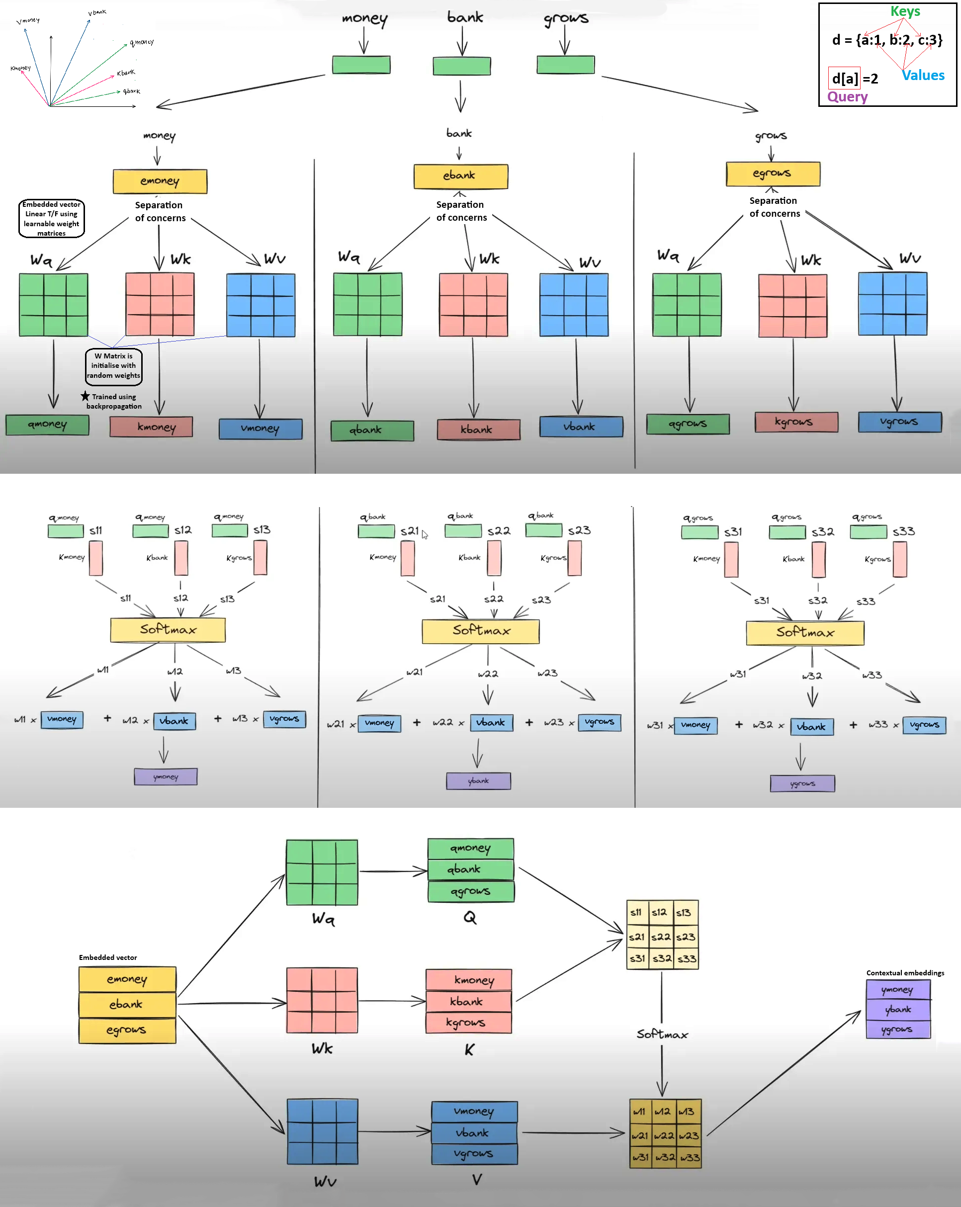
🔴 Separation of Concerns: By projecting the input embedding into Queries, Keys, and Values (Q, K, V), the network isolates the search criteria, the matching profile, and the actual content.
🔴 Task Adaptability: Learnable parameter matrices (\(W_Q, W_K, W_V\)) are refined during backpropagation, enabling the attention mechanism to specialize for specific downstream NLP tasks.
1. How Self-Attention Transforms Embeddings
Context-Aware Refinement: Unlike static word vectors, self-attention allows words to interact dynamically. For example, if "bank" is near "river", it pulls semantic context from the water-related dimension.
Global Affinity: Computes pairwise similarity scores between all tokens in a sentence using dot products, evaluating how strongly every word relates to every other word.
Normalized Weights: Raw similarity scores are passed through a Softmax function to convert them into positive attention weights that sum to 1.0.
Weighted Aggregation: The final contextual embedding is a weighted sum of the sequence's word vectors.
2. The Roles of Queries, Keys, and Values
To enable flexible and learnable context-extraction, each input token projects its embedding into three distinct vectors:
Query (Q) — The "Searcher": Represents the word's current search criteria. It "asks questions" of other words in the sentence to determine what context is relevant.
Key (K) — The "Responder": Acts as a descriptive profile or label for the word, matching against incoming Queries to evaluate relevance.
Value (V) — The "Information Provider": Contains the raw semantic information of the word. Once Q and K determine the relevance weights, the Values are scaled and summed.
Component Name
Description
Mathematical Representation
Role in Mechanism
Analogy Example
Learnable Parameters
Query (Q)
A transformed vector representing the word's search criteria or 'questions' it asks of other words.
qi = ei · WQ
Used to calculate similarity scores by performing dot products with key vectors of all words in the sequence.
The 'Search' criteria on a matrimonial site (e.g., looking for a partner with specific traits).
Yes (Weight matrix WQ)
Key (K)
A transformed vector representing the word's profile or characteristics against which queries are matched.
ki = ei · WK
Acts as a reference for queries to determine how much attention should be paid to this specific word.
The 'Profile' on a matrimonial site that other users see when they are searching.
Yes (Weight matrix WK)
Value (V)
A transformed vector containing the actual information of the word that will be aggregated into the final output.
vi = ei · WV
Represents the 'content' of the word; it is weighted by attention scores to form the contextual embedding.
The 'Match' or actual interaction/personality shared once a connection is established.
Yes (Weight matrix WV)
Contextual Embedding (Output)
The final dynamic representation of a word that incorporates information from its surroundings.
yi = Σj (wij · vj)
Provides a task-specific, context-aware vector that resolves ambiguities (e.g., distinguishing 'river bank' from 'money bank').
The refined understanding of a person after matching and filtering information through specific preferences.
No (Result of learned weights WQ, WK, WV)
Static Embedding (Input)
The initial numerical representation of a word that captures semantic meaning but lacks context.
Vector ei
Acts as the starting point for the transformation; the raw material from which Q, K, and V vectors are derived.
A person's raw information or life story as detailed in their autobiography.
Yes (Weights in embedding layer)
Dot Product (Similarity)
A mathematical operation used to quantify the relationship between a query and a key.
sij = qi · kj
Determines the raw attention score or affinity between words in a sequence.
Checking compatibility between a search query and a person's profile on the website.
No (Fixed mathematical operation)
Softmax
An activation function that normalizes raw similarity scores into probabilities that sum to 1.
wij = exp(sij) / Σk exp(sik)
Ensures the attention weights are positive and normalized, defining the percentage of influence each word has.
Allocating a finite amount of interest/attention across different potential profiles.
No (Fixed mathematical operation)
3. Learnable Projections & The Linear Formulas
Linear Projections: Multiplying raw static embeddings by weight matrices yields task-specific Query, Key, and Value representations.
Weight Matrices: The projection parameters (\(W_Q, W_K, W_V\)) are learned dynamically through training, allowing the model to adapt Q, K, and V distributions to the specifics of translation, classification, or generation tasks.
Q=WQ⋅X,K=WK⋅X,V=WV⋅X
4. Practice Questions & Concept Intuitions
Q1: How does self-attention project input embeddings into Query, Key, and Value vectors?
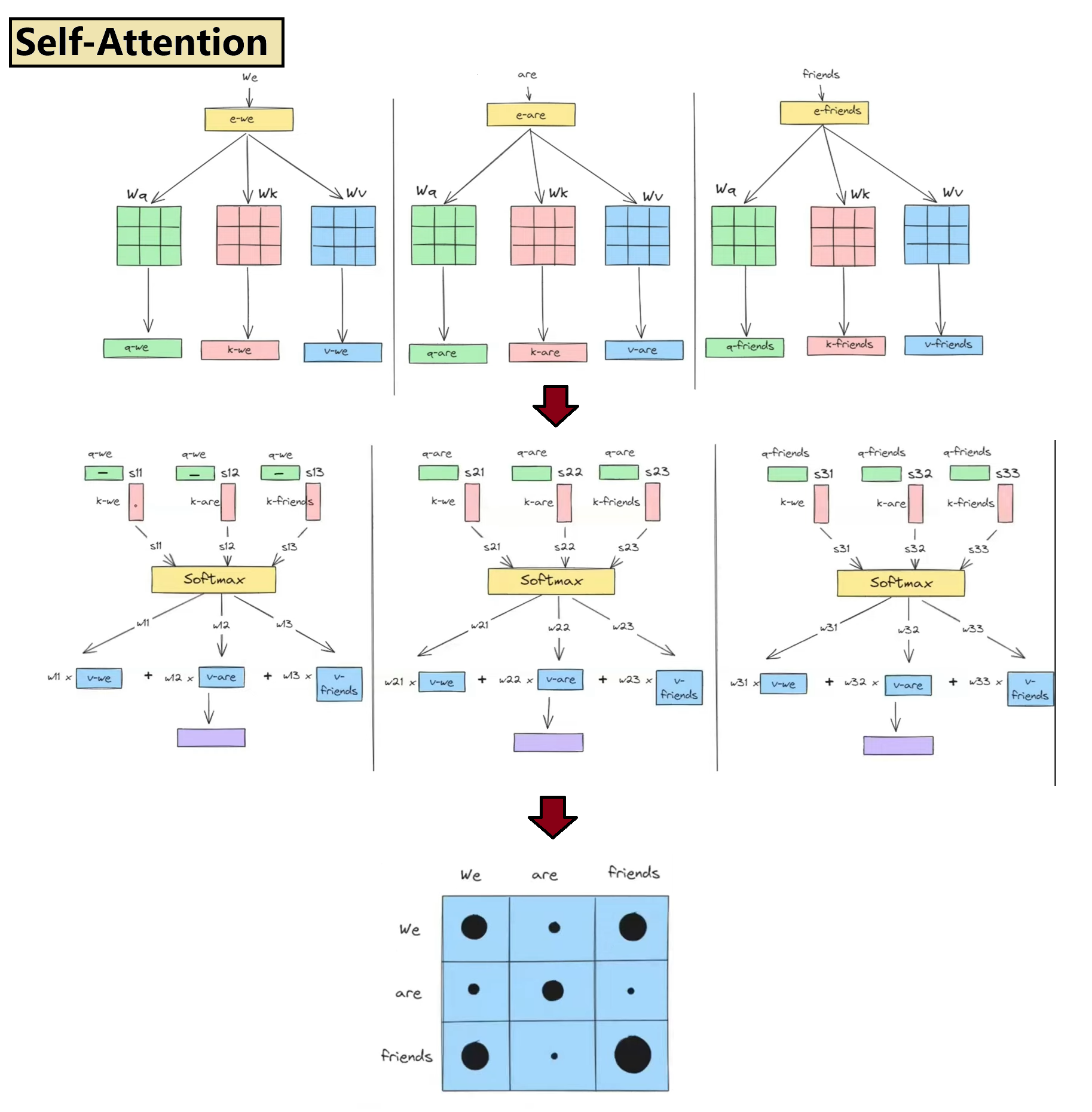
Linear Projections via Matrix Multiplication: The input embedding matrix \(X\) (shape \(N \times d_{\text{model}}\)) is multiplied by three separate learnable weight matrices: \(W_Q\) (shape \(d_{\text{model}} \times d_k\)), \(W_K\) (shape \(d_{\text{model}} \times d_k\)), and \(W_V\) (shape \(d_{\text{model}} \times d_v\)), yielding the projected matrices \(Q = X W_Q\), \(K = X W_K\), and \(V = X W_V\).
Creating Distinct Semantic Subspaces: Projecting the same input vector into three distinct spaces allows each representation to specialize in a specific relational role. A single token can seek context (Query), represent its matching attributes (Key), or hold its semantic content (Value) independently.
Dimensionality Adjustment: These projection matrices can scale the vector size up or down, allowing the model to adapt representation density to optimize computation (e.g., splitting the model dimension across multiple parallel attention heads).
Q2: What is the conceptual analogy of Query, Key, and Value in a database retrieval system?
Query (Search Input): Represents the search term you submit to a database (what information the current token is seeking to complete its meaning).
Key (Database Index Tags): Represents the index tags or identifiers of all records in the database. In self-attention, every token in the sequence exposes its Key to describe what features it can offer to a Query.
Value (Record Content): Represents the actual data stored in the matching records. Once the Query determines similarity with each Key, it retrieves a weighted blend of the corresponding Values to update its representation.
Q3: Why do we need learnable weight matrices (\(W_Q, W_K, W_V\)) in the attention mechanism?
Adapting Similarity Metrics: Without learnable matrices, attention would be a static calculation based on fixed input embeddings. Learnable weights allow the model to adjust representations based on training data, learning which feature matches are important for specific tasks.
Creating Specialized Representations: They project static embeddings into different dimensions, allowing the model to focus on syntactic structures (e.g., subject-verb alignment) in one head and semantic ties (e.g., pronoun resolution) in another.
Weight Optimization via Backpropagation: During training, gradients flow through the attention weights, continuously refining the projections to route information more accurately through the network layers.
Q4: What is the mathematical formula for computing self-attention?
The Core Equation: Self-attention is computed as:
\( \text{Attention}(Q, K, V) = \text{softmax}\left(\frac{Q K^T}{\sqrt{d_k}}\right) V \)
Scaled Similarity: The term \(Q K^T\) computes raw dot product similarities between all Query and Key pairs. The scaling factor \(1/\sqrt{d_k}\) scales the variance back to 1.0, keeping the Softmax function from saturating.
Weighted Value Assembly: The Softmax function converts similarity scores into a probability distribution. Multiplying this distribution by the Value matrix \(V\) builds a weighted sum of representation vectors.
Q5: Explain step-by-step how the raw attention scores are computed.
Step 1: Linear Projection: Multiply the input embedding matrix \(X\) by the projection weights \(W_Q, W_K\) to generate Query and Key matrices \(Q, K\) for all tokens in the sequence.
Step 2: Pairwise Dot Products: Compute the matrix multiplication \(Q K^T\). For each query \(q_i\) and key \(k_j\), this calculates a raw dot product similarity score \(s_{ij} = q_i \cdot k_j\), producing an \(N \times N\) matrix.
Step 3: Scaling: Divide every element in the similarity matrix by the scaling factor \(\sqrt{d_k}\) to suppress variance expansion in higher dimensions.
Q6: What is the role of the Softmax function in self-attention?
Probability Mapping: Softmax normalizes raw scaled scores along each row: \(\text{softmax}(z)_i = \exp(z_i) / \sum_j \exp(z_j)\). This maps real-valued scores into positive values between 0 and 1 that sum to exactly 1.0.
Attention Weight Assignment: The normalized scores represent the percentage of attention each query token should distribute to all key tokens in the sequence.
Differentiable Selection: By acting as a soft, continuous routing filter, Softmax allows gradients to flow back through all similarity paths, making the attention routing system fully end-to-end trainable.
Q7: How does Softmax normalization handle negative similarity scores?
Exponentiation to Positive: The Softmax function exponentiates its inputs: \(\exp(x)\). Since \(\exp(x) > 0\) for all real values of \(x\), any negative dot product is mapped to a positive value.
Relative Dampening: Large negative values map to numbers very close to 0 (e.g., \(\exp(-10) \approx 4.5 \times 10^{-5}\)), ensuring that unrelated tokens receive almost zero attention weight.
Smooth Transitions: Rather than hard-blocking negative matches (which would break gradient flow), Softmax smoothly dampens their weights while keeping the operation differentiable.
Q8: What is the physical interpretation of the Value vector weighting process?
Barycentric Context Blending: The final output is calculated as \(Y = A V\), where \(A\) is the attention weight matrix. Each output vector \(y_i\) is a weighted linear combination of all Value vectors in the sequence.
Information Filtering: The attention weights act as routing coefficients. Value vectors with high weights contribute heavily to the output vector, while low-weight values are ignored.
Dynamic Feature Assembly: This process pulls relevant features from context words and injects them into the target representation, constructing a context-aware token embedding.
Q9: How do Query, Key, and Value projections allow a single token to serve different roles?
Representational Partitioning: By using three independent projection matrices, a token's static representation is split into three separate vectors: Query, Key, and Value.
Decoupled Roles: This allows a token to seek context (using its Query), offer itself as a match (using its Key), and carry its content (using its Value) independently and simultaneously.
Flexible Routing: A word can actively attend to subject words in the sentence while serving as an important context object for verbs, without these roles interfering with one another.
Q10: Why would a token have a high similarity score with itself in self-attention?
Shared Semantic Origin: A token's Query and Key vectors are projected from the same underlying embedding vector, so they naturally share many semantic properties.
Identity Anchoring: This ensures that in the diagonal of the attention map (\(s_{ii} = q_i \cdot k_i\)), the scores remain high, allowing the token to retain its core identity.
Preventing Semantic Washout: Self-attention updates tokens by blending them with their context. High self-similarity ensures a token does not get completely overridden by context words and lose its original meaning.
Q11: How does self-attention enable the model to establish syntactic dependencies (e.g., matching verbs to nouns)?
Matching Syntactic Clues: Learnable weights allow the Query of a verb to project to features that align with the Keys of subject/object nouns, capturing structural grammar.
Directed Routing: During the dot product calculation, the verb token assigns high attention weights to its corresponding subject/object tokens, linking them in vector space.
Hierarchical Parsing: As signals pass through multiple layers, the model builds a hierarchical map of the sentence, resolving complex, nested clauses.
Q12: What would happen if we set \(W_Q, W_K, W_V\) to identity matrices?
No Projections: Q, K, and V would be identical to the input embedding matrix \(X\).
Static Similarity: Attention would rely strictly on the similarity of static embeddings, preventing the network from learning specialized query contexts or task-specific routing.
Loss of Expressive Power: The model would be unable to partition features across multiple parallel attention heads, severely limiting its capacity to capture different semantic perspectives.
Q13: How does self-attention scale computationally with the sequence length?
Quadratic Scaling: Computing similarity scores requires pairwise interactions between all tokens, resulting in \(O(N^2)\) operations and memory for a sequence of length \(N\).
Memory Bottleneck: Storing the \(N \times N\) attention weight matrices for large context windows (e.g., \(N > 32k\)) requires huge amounts of GPU memory, limiting context length.
Parallel Efficiency vs Scaling: Although highly parallelizable, the quadratic cost makes long-context training computationally expensive, prompting the development of linear-attention models.
Q14: How does the projection dimension (\(d_k\)) affect the representational capacity of Q, K, and V?
Expressive Power: Larger \(d_k\) allows Q, K, and V to represent more nuanced semantic features.
Subspace Balance: In Multi-Head Attention, we divide the model dimension by the number of heads: \(d_k = d_{\text{model}} / h\). This balances subspace detail against the number of parallel perspectives.
Q15: How do Queries, Keys, and Values interact to dynamically route information?
Affinity Matrix Construction: The dot product \(Q K^T\) builds a dynamic affinity matrix indicating how tokens relate to each other.
Softmax Filtering: Softmax acts as a gating filter, turning similarity scores into weights that sum to 1.0.
Weighted Routing: Multiplying this gated matrix by the Value matrix \(V\) dynamically routes information through the network, updating token representations based on context.
04 - Scaled Dot Product Attention
⭐ Overview
Scaled Dot-Product Attention is the core computational kernel of the Transformer architecture. It computes relationships between Queries and Keys, normalizes the scores, and aggregates Values. Crucially, it scales the dot products to maintain numerical stability during training.
💡
Problem:
High
variance is a problem because as the dimensionality
(dk) of the vectors increases, the variance of
the dot product also increases.This
causes the softmax function to assign very high probabilities to
large values and very low probabilities to small values. During
training, when updating the weight matrices (WQ,
WK, WV) using backpropagation, the
gradients are calculated to adjust the parameters. However,
backpropagation focuses more on larger values, assigning them
higher importance while ignoring smaller values. As a result,
some corresponding parameters experience vanishing gradients,
meaning their gradient values become extremely small. If these
gradients become too small, the parameters will not be updated
effectively, preventing proper learning. This leads to a poor
training process and an unstable self-attention mechanism.
Fix:
Scale the dot product
by dividing with √dk (dimension of key
vectors) to stabilize variance, ensuring balanced softmax
probabilities and gradients, preventing vanishing gradients.
1. The Scaling Factor in Self-Attention
Variance Control: The scaling factor \(1 / \sqrt{d_k}\) stabilizes the variance of the dot product results, preventing them from growing uncontrollably as the dimension \(d_k\) scales up.
Balanced Softmax: By curbing score magnitudes, the scaling factor keeps the Softmax operation from concentrating weight entirely on a single token, which would crush other values.
Gradient Stability: Helps prevent vanishing gradients, ensuring all parameters receive meaningful updates during backpropagation.
Attention(Q,K,V)=softmax(dkQ.KT)V
Here is a breakdown of why and how scaling is used:
Preventing Softmax Saturated Regions: As the key dimensionality \(d_k\) grows, the dot products grow in magnitude, producing high-variance distributions. Without scaling, Softmax outputs map to extreme probabilities (1.0 or 0.0), saturating the activation function.
Mitigating Vanishing Gradients: Saturated Softmax regions have near-zero local derivatives. Normalizing scores ensures that gradients flow back smoothly to Query, Key, and Value projection weights.
Variance Normalization: Dividing by \(\sqrt{d_k}\) scales the variance of the dot product back to exactly 1.0, keeping the distribution stable.
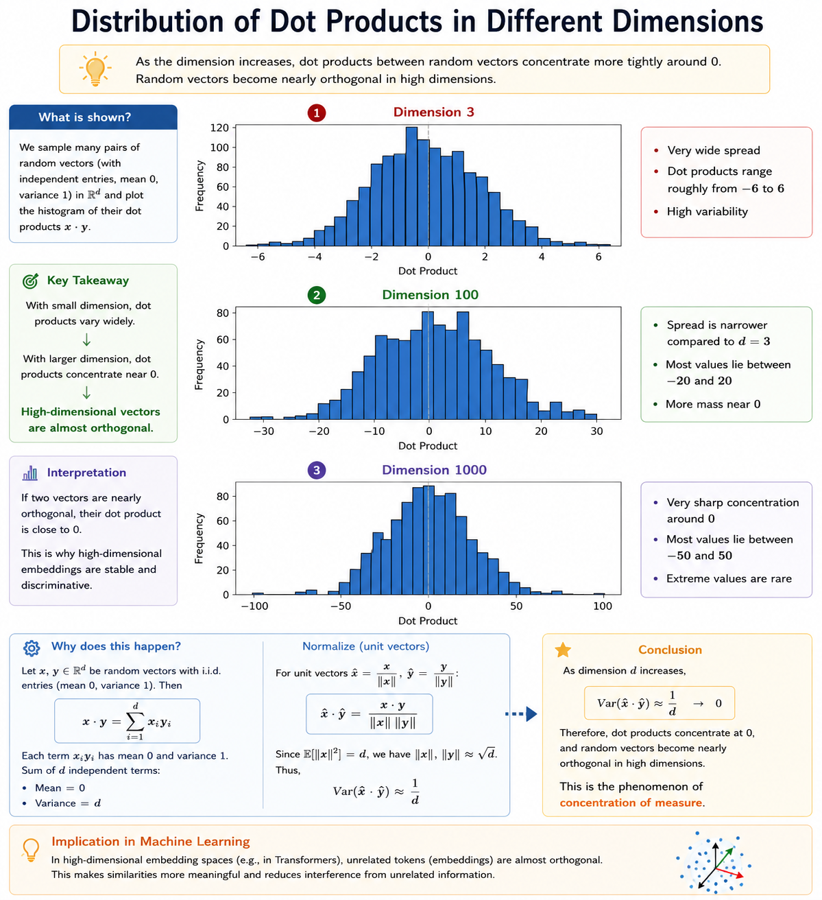
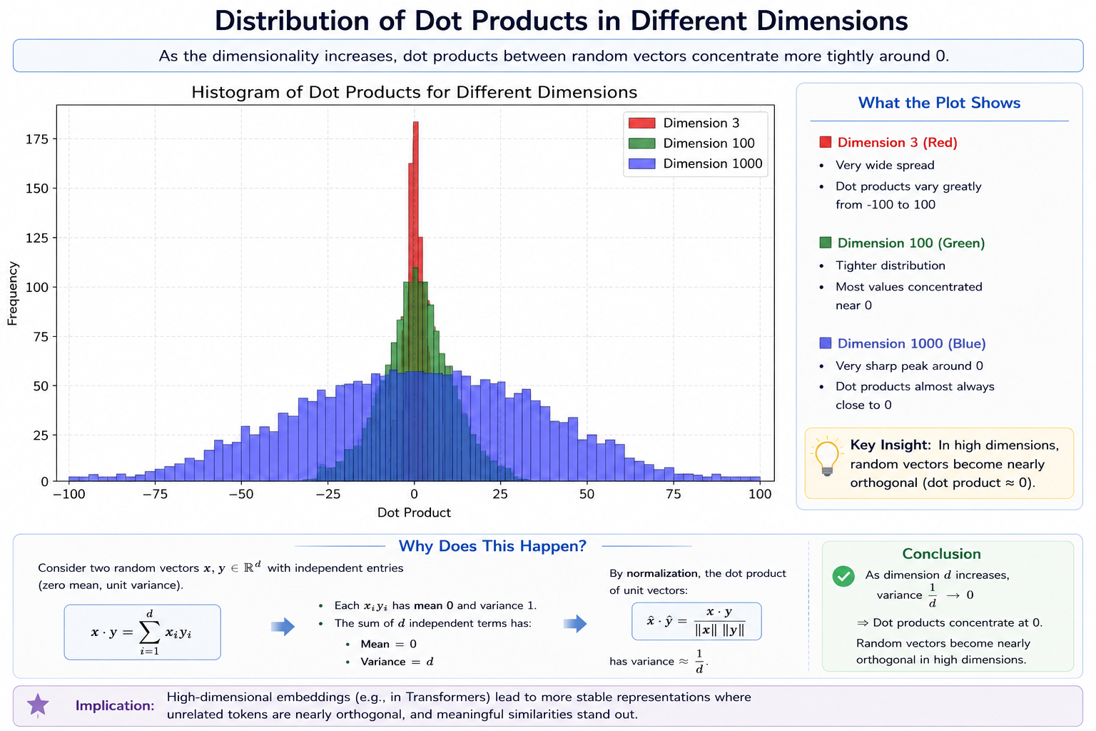
2. How Vector Dimensionality Affects Attention
The vector dimension \(d_k\) directly scales the range of raw dot products. Higher dimensions increase representation capacity but introduce statistical variance:
Low Dimension (e.g., \(d_k = 3\)): Dot products stay close to 0 with low variance, allowing Softmax to distribute attention weights evenly.
Medium Dimension (e.g., \(d_k = 100\)): The variance expands slightly, but Softmax remains active across multiple tokens.
High Dimension (e.g., \(d_k = 1000\)): Without scaling, dot products exhibit high variance. Extreme values dominate, leading to training instabilities.
3. High Dimensionality and Training Instability
The technical concept comparison table below details the interactions between dimensionality, variance, and the Softmax function:
Concept
Symbol
Definition
Role in Self-Attention
Mathematical Impact
Scaling
Factor
1 / √dk
The
factor used to divide the dot product scores
before applying the softmax function.
Stabilizes the variance of
the attention scores regardless of
dimensionality.
By dividing by
√dk, the variance
is brought back to a constant level, preventing
extreme softmax values and the vanishing
gradient problem.
Vector
Dimensionality
dk
The
dimensionality of the key vectors (and
query/value vectors in simplified setups).
Determines the complexity
and information capacity of the representations.
As dk increases,
the variance of the dot product
Q · KT increases
linearly (roughly dk times the
variance of a 1D vector).
Softmax
Function
softmax
An
activation function that converts a vector of
scores into a probability distribution totaling
1.
Normalizes attention scores
to determine the weights applied to the Value
matrix.
In the presence of high
variance, it assigns near 100% probability to
large values and near 0% to others, causing
vanishing gradients for smaller values.
Dot Product
Variance
Var(Q · KT)
The
statistical spread of the values resulting from
the dot product of high-dimensional vectors.
Indicates the range of
attention scores before scaling and softmax.
High variance leads to
extreme values (very large or very small), which
negatively impacts the softmax function's
behavior.
Vanishing Gradient
Problem
—
A
training issue where gradients become extremely
small, preventing parameter updates.
Result of extreme softmax
outputs caused by unscaled high-dimensional dot
products.
Training focuses only on
large values while small values are ignored,
leading to unstable or ineffective learning.
Key Matrix
K
A
matrix formed by stacking key vectors
(dk-dimensional) derived from
embeddings and the WK parameter
matrix.
Serves as the reference
against which queries are compared.
Its dimensionality
(dk) directly influences the variance
of the dot product; its transpose is multiplied
by Q.
Query
Matrix
Q
A
matrix formed by stacking query vectors
generated from the dot product of word
embeddings and the WQ parameter
matrix.
Used to interact with the
Key matrix to calculate attention scores.
Acts as the first operand
in the dot product operation to determine how
much attention one word should pay to others.
Value
Matrix
V
A
matrix consisting of value vectors that store
the actual information to be extracted.
Provides the content that
is weighted by the attention scores.
Multiplied by the result of
the softmax function to produce the final
contextual embeddings.
4. Probability Theory and the Variance Proof
Below is the detailed step-by-step mathematical proof of why dot product variance scales linearly with vector dimensionality, and how division by \(\sqrt{d_k}\) stabilizes it:
Probability theory regarding the variance
of a
scaled random variable:
Step-by-Step Explanation
Step 1:
Definition of Variance
The
variance of a
random variable X
is given by:
Var(X)=E[(X−E[X])2]
where:
E[X]
is the expected value (mean) of X
E[(X−E[X])2]
represents the expected squared deviation
from the
mean.
Step 2:
Define the Scaled Random Variable
We define
a new
random variable Y
as:
Y=cX
where
c
is a constant.
Step 3:
Compute the Mean of Y
Using the
linearity of expectation:
E[Y]=E[cX]=cE[X]
Step 4:
Compute the Variance of YY
By
definition:
Var(Y)=E[(Y−E[Y])2]
Substituting
Y=cXand
E[Y]=cE[X],
we get:
Var(cX)=E[(cX−cE[X])2]
Factor out
c:
Var(cX)=E[c2(X−E[X])2]
Since
expectation
is linear, we can take c2
outside:
Var(cX)=c2E[(X−E[X])2]
Since the
expectation inside is just the definition of variance:
Var(cX)=c2Var(X)
This
result shows
that when a random variable is scaled by a constant c,
its variance is scaled by c2,
which has applications in machine learning, deep learning,
and
signal processing.
Scaling
Key Mathematical Concepts:
Linear Growth of Variance:
The variance of
the dot
product of two random vectors scales
linearly with
the dimensionality d.
If
Var(x) is the
variance of
the dot product in one
dimension, then
in d dimensions:
Var(w⊤⋅x)=d⋅Var(x)
This
follows from the sum of
independent
random variables, assuming each
dimension contributes
additively.
Scaling Rule for Variance:
If
a random
variable x has
variance
Var(x), scaling by
a
constant c results
in:
Var(cx)=c2Var(x)
This is
fundamental in understanding
normalization techniques.
Justification for Scaling by
d1
:
Since
variance grows linearly with
d, normalizing by
d1
ensures that the variance
remains
stable:
Var(d1w⊤x)=d1⋅d⋅Var(x)=Var(x)
This is
commonly applied in
weight
initialization
(e.g.,
Xavier/Glorot initialization in
neural
networks) to keep activations
balanced.
5. Practice Questions & Concept Intuitions
Q1: What is the core mathematical function of Scaled Dot-Product Attention?
Mathematical Formulation: It is defined by the matrix formula:
\( \text{Attention}(Q, K, V) = \text{softmax}\left(\frac{Q K^T}{\sqrt{d_k}}\right) V \)
where \(Q\), \(K\), and \(V\) are the Query, Key, and Value matrices respectively, and \(d_k\) is the dimension of the key vectors.
The Dot-Product Operation: The product \(Q K^T\) computes pairwise dot products between all Queries and Keys, capturing raw similarity scores. For a sequence of length \(N\), this results in an \(N \times N\) compatibility matrix representing the raw alignment coefficients.
Softmax and Value Weighting: The softmax function is applied row-wise to convert these raw, scaled scores into attention weights (probabilities summing to 1.0). Multiplying by the Value matrix \(V\) computes a weighted linear combination of the value vectors, routing information dynamically based on relevance.
Q2: Why is the scaling factor \(\sqrt{d_k}\) introduced in self-attention?
Suppression of Variance Growth: As the key dimension \(d_k\) increases, the variance of the dot product between two independent, unit-variance vectors grows linearly as \(d_k\). Dividing by \(\sqrt{d_k}\) scales the variance back to a constant \(1.0\).
Mitigating Softmax Saturation: Without scaling, large dimensions yield high-magnitude dot products. These extreme values push the softmax function into flat, saturated regions where the output is dominated by a single key.
Preserving Backpropagation Gradients: Keeping the input variance to the softmax stable prevents its gradients from vanishing, which guarantees smooth and stable gradient flow back to the projection layers during training.
Q3: What is "softmax saturation" and how does it relate to vector dimensionality?
Mechanics of Saturation: Softmax saturation occurs when the input elements have large absolute differences. The exponential nature of the softmax function drives the output probability of the largest element near \(1.0\) and all others to near \(0.0\).
Role of High Dimensionality: In higher-dimensional spaces (larger \(d_k\)), the dot product sum has many more terms, naturally widening the distribution and increasing the likelihood of producing extremely large positive and negative values.
Loss of Soft Information: A saturated softmax converts attention into a hard selection (similar to argmax), preventing the model from aggregating information from multiple context-relevant tokens simultaneously.
Q4: How does softmax saturation lead to the vanishing gradient problem?
Flat Derivative: The derivative of a softmax output \(s_i\) with respect to its input \(z_j\) is \(s_i(\delta_{ij} - s_j)\). When \(s_i\) approaches \(1.0\) (or \(0.0\)), the derivative product \(s_i(1 - s_i)\) becomes virtually zero.
Interruption of Gradient Flow: During backpropagation, upper-level gradients are multiplied by this near-zero Jacobian matrix, preventing errors from propagating to earlier query, key, and value projection matrices.
Freeze of Weight Updates: This effectively freezes the learning process for the projection parameters, stopping the model from adapting its attention patterns and stalling convergence.
Q5: Outline the core assumption in the proof that the dot product variance is \(d_k\).
Independent Random Variables: The components of the Query vector \(q\) and Key vector \(k\) are assumed to be independent, meaning there is no correlation between \(q_i\) and \(k_j\) for all indices \(i, j\).
Standard Normal Distribution: Each component is assumed to be drawn from a standard normal distribution with mean \(\mu = 0\) and variance \(\sigma^2 = 1.0\), giving \(\mathbb{E}[q_i] = \mathbb{E}[k_i] = 0\) and \(\text{Var}(q_i) = \text{Var}(k_i) = 1.0\).
Summation of Variances: The dot product is \(\sum_{i=1}^{d_k} q_i k_i\). Since individual product terms \(q_i k_i\) are independent and have variance \(\text{Var}(q_i k_i) = 1.0\), the variance of the sum is the sum of the variances, which equals \(d_k\).
Q6: Why does a variance of \(d_k\) cause the inputs to the softmax function to have large magnitudes?
Standard Deviation Spread: A variance of \(d_k\) translates to a standard deviation of \(\sqrt{d_k}\). For a standard key dimension of \(d_k = 512\), the standard deviation of dot products is \(\sqrt{512} \approx 22.63\).
Broad Ranges of Values: Since the values span a range proportional to the standard deviation, it is highly probable that some dot products will be extremely large positive values (e.g., \(+40\)) and others extremely negative.
Softmax Input Disparity: Feeding these widely spread values to the exponential operators inside the softmax causes the largest values to completely dominate, causing rapid saturation.
Q7: How does scaling the dot product by \(1/\sqrt{d_k}\) affect the variance?
Variance Quadratic Scaling Rule: For any random variable \(X\) and constant scaling factor \(c\), the variance of the scaled variable is \(\text{Var}(cX) = c^2 \text{Var}(X)\).
Application to Attention: Setting \(c = \frac{1}{\sqrt{d_k}}\) and \(X = q \cdot k\), we get:
Stabilizing Scale: By forcing the variance of the attention scores to remain exactly \(1.0\) regardless of the key dimension \(d_k\), the values remain centered in the active, high-gradient range of the softmax function.
Q8: Why not scale by \(d_k\) instead of \(\sqrt{d_k}\)?
Under-dispersion and Variance Compression: Scaling by \(d_k\) would reduce the variance of the dot product to \(\frac{1}{d_k^2} \cdot d_k = \frac{1}{d_k}\). For \(d_k = 512\), the variance becomes \(\frac{1}{512} \approx 0.00195\).
Softmax Flattening Effect: A variance this low means all dot products are compressed extremely close to zero, forcing the softmax output to distribute weight almost uniformly (approx. \(1/N\) for all tokens).
Loss of Focus: Uniform attention weights prevent the model from learning target-specific features, effectively reducing the self-attention mechanism to a basic average pooling step.
Q9: What is the physical role of the Value matrix in Scaled Dot-Product Attention?
Information Payload: While Queries and Keys determine *where* to pay attention (the routing matrix), the Value matrix \(V\) represents *what* information to retrieve and propagate.
Contextual Weighted Assembly: Multiplying the softmax attention distribution by the Value matrix yields a weighted sum of representation vectors, producing the final contextualized token embeddings.
Representation Decoupling: Keeping the Value projection separate from Queries and Keys allows the model to learn routing patterns independently of the features being routed.
Q10: How does Scaled Dot-Product Attention handle variable sequence lengths?
Length-Independent Scaling: Because the scaling factor \(\sqrt{d_k}\) depends strictly on key dimensionality and not sequence length \(N\), the statistical properties of the dot product remain stable.
Attention Masking: For shorter sequences in a batch, padding tokens are masked out by adding a large negative value (e.g., \(-10^9\)) to their raw attention scores before softmax, forcing their attention weights to zero.
Consistent Probability Ranges: This ensures that even as sequence length changes, the active non-masked tokens maintain a mathematically balanced attention distribution.
Q11: Explain the numerical overflow and underflow risks in unscaled attention.
Overflow in Low Precision: In mixed-precision training (like float16), the maximum representable value is \(65,504\). High-dimensional unscaled dot products can easily exceed this limit, causing overflow and producing `NaN` values.
Underflow and Information Loss: Saturated softmax drives smaller weights down to the precision limit of the floating-point system, rounding them to absolute zero and losing subtle semantic connections.
Numerical Safeguarding: Scaling by \(\frac{1}{\sqrt{d_k}}\) centers values near a standard deviation of 1.0, keeping calculations well within standard numerical precision bounds.
Q12: How is Scaled Dot-Product Attention computed in parallel using GPU tensors?
Batched Matrix Multiplication (BMM): Queries, Keys, and Values are represented as 3D tensors. The multiplication \(Q K^T\) is computed in parallel across batches and heads using optimized GPU GEMM (General Matrix Multiply) operations.
Parallel Kernel Execution: Division by \(\sqrt{d_k}\), masking, and softmax operations are performed element-wise in parallel across GPU threads using highly optimized CUDA kernels.
Value Combination: The attention weight matrix is multiplied by the Value tensor in a final batched multiplication, producing the final contextualized outputs simultaneously for all tokens.
Q13: How does the scaling factor affect convergence rate during training?
Smooth Gradients: Preventing softmax saturation ensures that gradients flowing back to early layers remain stable, rather than vanishing or exploding.
Higher Learning Rates: Since gradient magnitudes are well-behaved, optimizers can utilize larger learning rates without destabilizing training.
Reduced Training Time: Stable gradients lead to faster convergence, significantly reducing the number of optimization steps required to reach low loss.
Q14: Describe an alternative scaling method to \(1/\sqrt{d_k}\) and its trade-offs.
Learnable Temperature: Some models replace the static factor \(\frac{1}{\sqrt{d_k}}\) with a learnable parameter \(\tau\), computing attention as \(\text{softmax}\left(\frac{Q K^T}{\tau}\right) V\).
Flexibility vs. Complexity: This permits the model to adjust attention entropy dynamically per head, but it increases the number of parameters and introduces extra optimization complexity.
Risk of Instability: If \(\tau\) is poorly initialized or becomes too small, it can trigger sudden softmax saturation and lead to vanishing gradients.
Q15: How does key dimensionality scale in massive LLMs (e.g., LLaMA), and why is scaling critical there?
Head-Wise Splitting: In massive models, the hidden dimension is large (e.g., 8192 in LLaMA-2 70B), but it is divided across many heads, typically keeping the head key dimension \(d_k\) at 128.
Need for Scaling at \(d_k = 128\): An unscaled key dimension of 128 would still yield a variance of 128 (standard deviation \(\approx 11.3\)), which is more than enough to saturate the softmax function.
Critical Role in Stability: In multi-billion parameter models, even a minor gradient vanish or numerical anomaly can derail the training run. Thus, scaling remains an absolute requirement for successful pre-training.
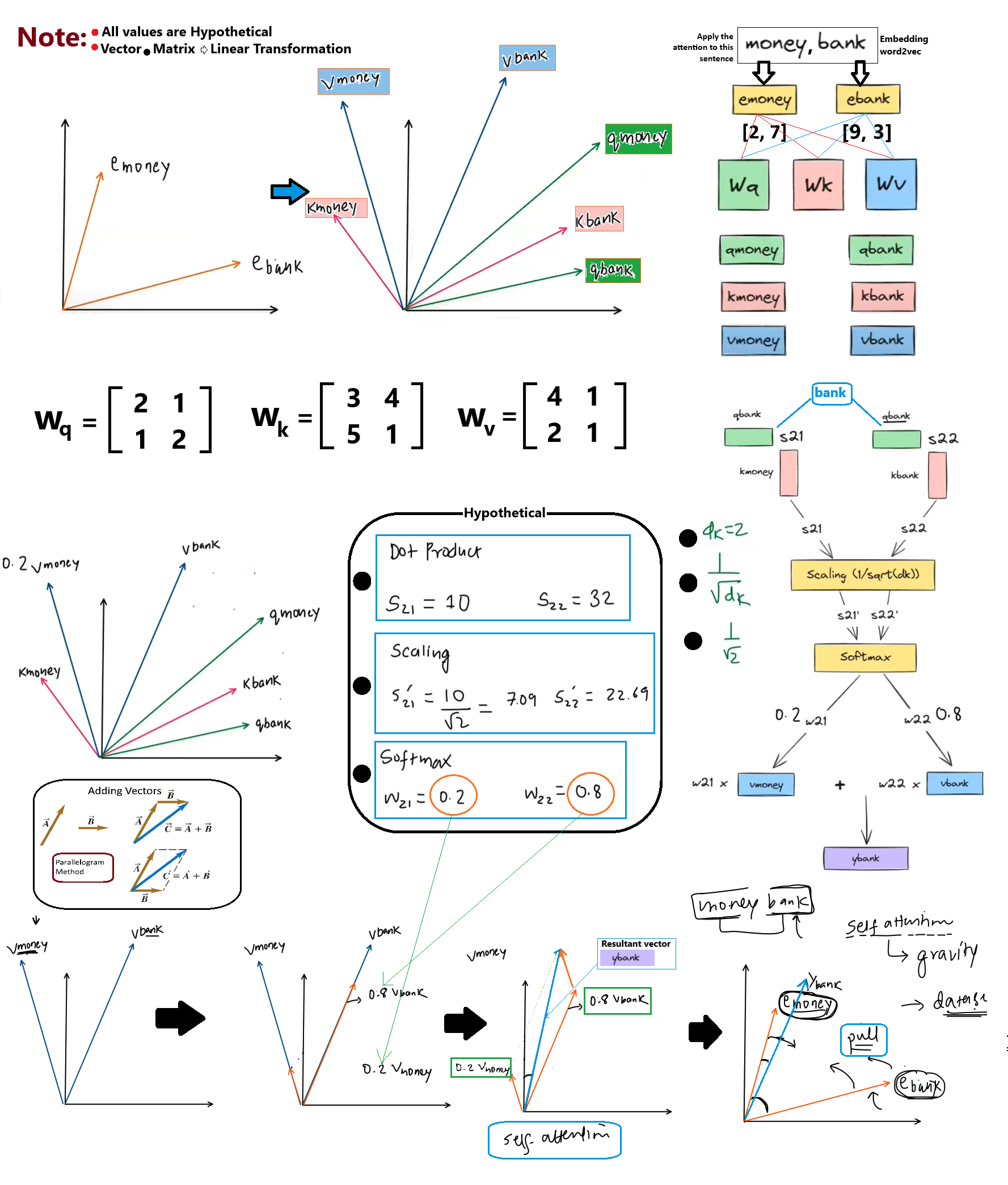
05 - Self-Attention Geometric Intuition
⭐ Overview
Self-attention operates as a geometric transformer in multi-dimensional space. By projecting word embeddings into Query, Key, and Value spaces, it measures angular alignments and constructs contextual representations through vector addition.
The "river bank" example demonstrates how the static representation of a word dynamically shifts toward relevant neighboring vectors based on context.
Concept
Vector/Matrix Symbol
Role in Self-Attention
Geometric Description
Mathematical Operation
Word Embeddings
E (e.g.,
Emoney, Ebank)
Initial
numerical representation of words serving as the starting point
for the mechanism.
Vectors
in a multi-dimensional space where semantic meaning is captured
by position.
Extracted via techniques like Word2Vec; plotted as points or
arrows in space.
Transformation Matrices
WQ,
WK, WV
Learnable parameters used to project word embeddings into
specific functional spaces (Query, Key, Value).
Act as
operators for linear transformation, moving or rotating vectors
to new locations.
Matrix
Multiplication (Dot Product with the embedding vector).
Query, Key, and Value
Vectors
q,
k, v (e.g.,
qmoney, kbank)
Functional components: Query searches, Key is matched against,
and Value contains the actual content.
Six new
vectors generated from the original word embeddings through
linear projection.
q = E · WQ;
k = E · WK;
v = E · WV
Similarity/Attention
Scores
s (or Score)
Measures the relevance or relatedness between words in the
sentence.
Based on
the angular distance between vectors; smaller angles result in
higher scores.
Dot
product of Query and Key vectors (q · k).
Scaling and Normalization
Softmax,
∑w = 1
Prevents vanishing/exploding gradients and converts similarity
scores into probabilistic weights.
Mapping
raw scores to a range that determines how much "pull" one word
has on another.
Division by √dk followed by the
Softmax function.
Weighted Sum/Attention
Output
y (e.g.,
ybank)
The
final contextual embedding of a word, influenced by all other
words in the sequence.
Resultant vector from scaling Value vectors and adding them;
acts like "gravity" pulling words toward relevant contexts.
Scalar
multiplication of Value vectors by weights, followed by Vector
Addition (Parallelogram/Triangle Law).
1. Word Embeddings in Multi-Dimensional Space
Given the sentence “money, bank”, the words are mapped to initial static vectors:
Semantic Coordinates: Each word exists as a vector pointing away from the origin in a high-dimensional space.
Initial Distance: Because "money" and "bank" are semantically distinct, their initial vectors (\(e_{\text{money}}\) and \(e_{\text{bank}}\)) point in different directions.
2. Transformation Matrices & Linear Projection
To compute attention, static embeddings are projected into functional spaces via linear transformations:
Linear Projections: Multiplying embeddings by these learnable matrices rotates, scales, and shears the vectors.
Query Space: Maps embeddings to \(q_{\text{money}}\) and \(q_{\text{bank}}\).
Key Space: Maps embeddings to \(k_{\text{money}}\) and \(k_{\text{bank}}\).
Value Space: Maps embeddings to \(v_{\text{money}}\) and \(v_{\text{bank}}\).
3. Geometric Meaning of Queries, Keys, and Values
Query (Q) — The Search Direction: Points in the direction of the information the word is actively seeking.
Key (K) — The Semantic Profile: Represents the word's characteristics. The alignment between a Query vector and a Key vector measures their contextual relevance.
Value (V) — The Content Payload: Represents the raw semantic information that will be blended to form the final contextual representation.
4. Attention Scores & Dot Product Alignment
We compute similarity scores for the word "bank" by measuring its Query alignment with all Keys:
Geometric Proximity: The dot product calculates the angular alignment between Query and Key vectors.
Self-Attention Bias: Since \(s_{22} > s_{21}\), \(q_{\text{bank}}\) is more aligned with \(k_{\text{bank}}\), meaning it initially pays more attention to itself.
5. Scaling and Softmax Normalization
Dividing by \(\sqrt{d_k} = \sqrt{2}\) normalizes the attention scores prior to Softmax:
Vector Blending: The resulting contextual vector \(y_{\text{bank}}\) points closer to \(v_{\text{bank}}\) in space, but is pulled slightly in the direction of \(v_{\text{money}}\).
Gravity Analogy: Attention acts as semantic gravity. Tokens with high Query-Key alignment pull the final representation toward their semantic coordinates.
7. Practice Questions & Concept Intuitions
Q1: How do we interpret word embeddings geometrically in multi-dimensional space?
Vector Space Representation: Each word in a vocabulary is mapped to a high-dimensional vector, representing coordinates in an embedding space (e.g., \(d_{\text{model}} = 512\)). We interpret these vectors as arrows originating from the origin and pointing to a unique position in this hyperspace.
Semantic Proximity: Words that share semantic meanings, context, or syntactic functions are clustered together. Their vectors point in similar directions, resulting in small angular distances (high cosine similarity).
Spatial Dimensions as Concepts: Individual dimensions or combinations of dimensions represent abstract linguistic attributes (e.g., gender, verb tense, animacy), allowing algebraic operations like \(v_{\text{king}} - v_{\text{man}} + v_{\text{woman}} \approx v_{\text{queen}}\).
Q2: What is the geometric meaning of linear projection using matrices \(W_Q, W_K, W_V\)?
Space Transformation: Multiplying input vectors by the learnable weight matrices \(W_Q, W_K, W_V\) applies linear transformations (rotation, scaling, reflection, or shearing) to the original embedding space.
Role-Specific Subspaces: This maps the static input representation into three separate functional subspaces: the Query subspace (seeking context), the Key subspace (describing content to be matched), and the Value subspace (containing the information payload).
Dynamic Contextual Focus: Linear projection allows the model to alter which geometric features are relevant for attention scoring. For instance, the projection can isolate syntactic relationships in one attention head while focusing on semantic categories in another.
Q3: Geometrically, what does the Query vector represent?
Direction of Active Search: A Query vector \(q_i\) represents a probe or search direction in the Query subspace. It defines what semantic or syntactic properties the token \(i\) is currently seeking from other tokens in the sequence.
Targeted Linguistic Inquiry: The coordinates of \(q_i\) reflect a specialized query, such as "look for a direct object" or "find a matching pronoun," expressed as a specific coordinate direction.
Similarity Reference Point: Geometrically, it acts as a reference vector. When we compute the dot product with Key vectors, we measure the length of their projections along this specific query direction.
Q4: Geometrically, what does the Key vector represent?
Semantic Index Coordinate: A Key vector \(k_j\) represents the index coordinate of token \(j\) in the Key subspace, defining the specific features or "information profile" that this token offers to the rest of the sequence.
Landmark for Query Matching: It acts as a static geometric landmark. Queries from other tokens are compared against this landmark to evaluate compatibility.
Search Key Alignment: The orientation of the Key vector determines how strongly it will respond to different Query directions. If a Query's direction aligns closely with a Key's direction, the dot product will be maximized.
Q5: Why is the dot product used as a similarity measure in self-attention?
Projection Magnitude: The dot product \(q \cdot k\) measures the projection of vector \(q\) onto vector \(k\). It captures both the angular alignment (direction) and the magnitudes of the vectors.
Directional Agreement: When two vectors point in similar directions, their dot product is large and positive, indicating high similarity. If they are orthogonal (perpendicular), the dot product is exactly 0, signifying no relationship.
Computational Efficiency: Algebraically, the dot product involves simple element-wise multiplication followed by summation. This operation is highly parallelizable and executes extremely fast on modern GPU architectures via matrix multiplication.
Q6: How does the dot product relate to the angle between two vectors?
Geometric Definition: The dot product of two vectors \(q\) and \(k\) is mathematically defined as \(q \cdot k = \|q\| \|k\| \cos(\theta)\), where \(\|q\|\) and \(\|k\|\) are the Euclidean norms (lengths) and \(\theta\) is the angle between them.
Cosine Similarity Connection: If the vectors are normalized to unit length (\(\|q\| = \|k\| = 1\)), the dot product is exactly equal to the cosine of the angle \(\theta\).
Angular Interpretation: A cosine of \(1\) (\(\theta = 0^\circ\)) represents perfect alignment, a cosine of \(0\) (\(\theta = 90^\circ\)) indicates orthogonality, and a cosine of \(-1\) (\(\theta = 180^\circ\)) represents complete opposite directions.
Q7: What does a negative dot product mean geometrically, and how does Softmax handle it?
Divergent Orientations: Geometrically, a negative dot product indicates that the Query and Key vectors point in opposing directions (the angle \(\theta\) between them is greater than \(90^\circ\)), suggesting semantic incompatibility.
Softmax Non-Negativity: The softmax function applies the exponential function \(e^x\) to the scaled scores. This maps any negative score to a positive real number between \(0\) and \(1\), preventing negative probabilities.
Suppression of Irrelevant Context: Since \(e^x \to 0\) as \(x \to -\infty\), a negative dot product results in a very small numerator, forcing the final attention weight to be near \(0\) and effectively ignoring the opposing token.
Q8: Geometrically, what does the Value vector represent?
Semantic Information Content: The Value vector \(v_j\) represents the actual coordinate location of token \(j\)'s semantic information in the Value subspace, representing the "message" that will be transmitted.
Payload Representation: Unlike Queries and Keys, which are strictly used for routing and calculating similarity, the Value vector acts as the content payload to be blended and passed forward.
Contribution Coordinates: Geometrically, it defines the direction and magnitude of the vector contribution that token \(j\) will make to the final aggregated token representation.
Q9: How is the final contextual vector computed geometrically?
Linear Vector Combination: The final contextual representation \(y_i\) is computed as a weighted linear combination of all Value vectors: \(y_i = \sum_j w_{ij} v_j\).
Weighted Center of Gravity: Because the attention weights \(w_{ij}\) are positive and sum to \(1.0\), this calculation represents a convex combination, defining a weighted center of gravity (barycenter) within the convex hull of the Value vectors.
Coordinates Shift: The resultant vector \(y_i\) is pulled closest to the Value vectors that received the highest attention weights, shifting its coordinates to reflect the dominant contextual influences.
Q10: What is the "parallelogram law of vector addition" and how does it apply to self-attention?
Geometric Addition: The parallelogram law states that the sum of two vectors \(A\) and \(B\) is represented by the diagonal of the parallelogram formed with \(A\) and \(B\) as adjacent sides.
Multi-Vector Blending: In self-attention, we scale multiple Value vectors by their attention weights (which adjusts their lengths) and add them sequentially, constructing a multi-dimensional path whose final coordinate represents the blended sum.
Synthesizing Meaning: Adding scaled vectors merges their features. For example, adding the scaled vector for "bank" to the scaled vector for "river" creates a diagonal vector pointing to the specific concept of a "river bank".
Q11: Explain the concept of semantic "gravity" or "pull" in self-attention.
Attraction Poles: When a token's Query highly aligns with another token's Key, a large attention weight is generated. This creates a semantic "attraction pole."
Gravitational Vector Pull: The weighted summation pulls the output vector's coordinate direction toward the coordinates of the highly attended Value vectors, acting like semantic gravity.
Contextual Transformation: Through this pull, the static representation of a token dynamically relocates in vector space, adopting the characteristics of its semantic neighbors.
Q12: How do linear projections prevent the attention mechanism from being a simple, static nearest-neighbor search?
Dynamic Space Remapping: Without the learnable projections \(W_Q, W_K, W_V\), attention similarity would depend purely on the static cosine distance of the input word embeddings.
Contextual Flexibility: Projection matrices allow the model to project the same word into completely different locations depending on whether it acts as a Query, Key, or Value, allowing heads to capture diverse relational structures.
Task-Specific Subspaces: It transforms a static nearest-neighbor lookup into a learnable, task-dependent matching system, letting the model learn what features (tense, gender, position) to prioritize.
Q13: What happens to the geometry if two key vectors are orthogonal to a query vector?
Zero Alignment Projection: If key vectors \(k_1\) and \(k_2\) are orthogonal to query vector \(q\), their dot products are exactly zero: \(q \cdot k_1 = q \cdot k_2 = 0\).
Uniform Probability Distribution: If all keys in a sequence are orthogonal to the query, the softmax input vector will consist of zeros (or equal values), resulting in a uniform attention distribution where each token receives an equal weight of \(1/N\).
Geometric Indecision: Geometrically, this means the query vector cannot find any directional affinity in the key space, causing the model to default to a simple average pooling of the Value vectors.
Q14: How does the dimensionality of the vector space influence the geometric separation of concepts?
High-Dimensional Orthogonality: In high-dimensional spaces (e.g., \(d = 512\) or \(1024\)), random vectors are almost always nearly orthogonal.
Capacity for Disjoint Concepts: This geometric property provides vast space to distribute thousands of independent concepts, grammatical rules, and semantic classes with minimal interference.
Clean Separation Boundary: The vast volume of high-dimensional space enables linear classifiers and projection heads to easily separate and route distinct semantic ideas.
Q15: Geometrically, how does self-attention resolve lexical ambiguity (e.g., distinguishing "river bank" vs "money bank")?
Static Embedding Centroid: The word "bank" has a static embedding that initially sits at an ambiguous coordinate between the "financial" and "geographical" clusters in vector space.
Context-Driven Vector Pull: If the surrounding context contains the word "river", the Query for "bank" matches the Key of "river". This assigns a high weight to the Value vector of "river", pulling the output representation of "bank" into the geographical region of the space.
Disambiguated Coordinates: The final contextualized vector for "bank" is dynamically shifted away from its ambiguous origin to a specific, disambiguated location, representing the correct meaning.
Multi-Head Attention extends self-attention by performing the attention operation in parallel across multiple lower-dimensional subspaces. This allows the model to simultaneously process different perspectives of a sequence.
Mechanism Name
Key Objective
Weight Matrices Used
Handling of Perspectives
Output Dimension Compatibility
Main Advantage
Limitations
Self-Attention
To generate
contextual embeddings by capturing semantic meaning and word
relationships within a sentence.
One set
of weight matrices: \(W_Q\) (Query), \(W_K\) (Key), and \(W_V\)
(Value).
Captures only a single perspective or interpretation of a
document or sentence.
Produces a single contextual
representation; shape typically matches the input embedding.
Generates
contextual embeddings that solve the problem of static
embeddings where words have the same value regardless of
context.
Inability to
capture multiple linguistic perspectives or handle ambiguity
simultaneously.
Multi-Head
Attention
To capture
multiple different perspectives or hidden meanings in a sentence
simultaneously by using parallel attention modules.
Multiple
sets of \(W_Q\), \(W_K\), and \(W_V\) matrices (one set per
head) and a final output matrix \(W_O\).
Manages multiple perspectives by having each "head" focus on
different semantic or syntactic relationships.
Outputs from all heads are concatenated and
linearly transformed using \(W_O\) to match the input dimension.
Allows the
model to focus on different positions and perspectives at once;
improves summarization and disambiguation with high
computational efficiency.
Requires final
linear projection overhead (\(W_O\)) and additional parameter
calculation layers.
1. Dimension Changes & Vector Shapes
Input Embeddings: Words (e.g., "Money", "Bank") are mapped to standard \(d_{\text{model}} = 512\) vectors. For a sequence length of 2, the input matrix has a shape of \(2 \times 512\).
Subspace Projection: Input embeddings are multiplied by three projection matrices per head: \(W_Q, W_K, W_V\).
Head Dimension Splits: For \(h = 8\) heads, each head projects vectors to \(d_k = d_{\text{model}} / h = 64\) dimensions. Thus, projection matrices have shape \(512 \times 64\), yielding outputs of shape \(2 \times 64\) per head.
Concatenation: The \(2 \times 64\) outputs from all 8 heads are concatenated side-by-side, restoring the original dimension size: \(2 \times (64 \times 8) = 2 \times 512\).
Final Projection: The concatenated output is multiplied by a learnable matrix \(W^O\) of shape \(512 \times 512\) to blend the representations from all heads back into the final contextual sequence.
2. Computational & Memory Efficiency
Subspace Computation: Splitting vectors into 8 independent heads of 64 dimensions is computationally identical in terms of floating-point operations (FLOPs) to computing a single 512-dimensional attention head.
Complexity Math: A single large attention computation scales as \(O(d_{\text{model}}^2)\). For Multi-Head Attention, computing \(h\) independent operations yields:
This reduces dot-product calculation overhead by a factor of \(h\), freeing up memory.
GPU Parallelization: Because attention heads are independent, GPUs compute all head projections in parallel, accelerating training and inference.
3. Multi-Perspective Semantic Capture
Subspace Specialization: Different heads specialize in different relational aspects:
Head 1: Tracks local subject-verb syntax (e.g., matching "cat" to "sat").
Head 2: Tracks long-range pronouns (e.g., linking "mat" to "it").
Head 3: Evaluates modifier-noun relationships.
Lexical Disambiguation: Multiple heads allow the model to capture polysemy (e.g., distinguishing between a financial "bank" and a river "bank" simultaneously by attending to different surrounding context tokens).
4. Limitations of Self-Attention Resolved
Avoiding Over-Smoothing: Single-head self-attention tends to blend all syntactic and semantic relationships into a single average vector. Multi-head splits prevent feature homogenization.
Short and Long Range Tracking: Multi-head attention resolves the struggle of a single head to track both local grammatical relationships and global document structure at the same time.
Unresolved Quadratic Scaling: Although Multi-Head Attention optimizes dimension computation, the pairwise token comparisons still scale quadratically as \(O(N^2)\) with sequence length \(N\).
5. Practice Questions & Concept Intuitions
Q1: What is the fundamental difference between single-head Self-Attention and Multi-Head Attention?
Single-Head Constraints: Single-head self-attention computes a single set of attention scores across the full hidden dimension \(d_{\text{model}}\). This limits the model to focusing on one relationship pattern per token at a time (e.g., attending only to the subject and missing the object).
Multi-Head Subspaces: Multi-head attention splits the queries, keys, and values of the hidden dimension into \(h\) lower-dimensional subspaces, each of size \(d_k = d_{\text{model}} / h\). Each subspace runs attention in parallel, allowing different heads to specialize in different types of relations.
Perspective Diversity: This division allows the model to simultaneously capture different semantic, syntactic, and long-range dependencies, merging these distinct viewpoints into a richer, multi-faceted token representation.
Q2: Why do we project the input embeddings into lower-dimensional subspaces for each head?
Forced Head Specialization: Lower-dimensional projections restrict the representation capacity of each individual head. This forces them to focus on a narrow subset of features (like specific grammatical cases or gender markers) rather than trying to model all relationships at once.
Computational Efficiency: By dividing the query, key, and value vectors of size \(d_{\text{model}}\) into \(h\) chunks of size \(d_k = d_{\text{model}} / h\), the total computational complexity remains comparable to a single head operating on the full dimension, keeping the model fast.
Enabling Parallelism: Subspace projections create independent, head-specific matrices \(Q_i\), \(K_i\), and \(V_i\) that can be computed simultaneously on modern GPU cores using efficient parallel block matrix multiplications.
Q3: What are the mathematical shapes of Query, Key, and Value matrices for each attention head?
Projection Weight Shapes: The projection weight matrices for a single head \(i\)—denoted as \(W_i^Q\), \(W_i^K\), and \(W_i^V\)—have shapes of \(d_{\text{model}} \times d_k\) (or \(d_{\text{model}} \times d_v\)), where \(d_k = d_{\text{model}}/h\). For example, if \(d_{\text{model}}=512\) and \(h=8\), the shape is \(512 \times 64\).
Sequence Matrix Shapes: For an input sequence matrix \(X\) of shape \(N \times d_{\text{model}}\) (where \(N\) is the sequence length), multiplying by the weight matrices yields Query, Key, and Value tensors of shape \(N \times d_k\) (or \(N \times d_v\)) for each head.
Attention Map Shape: The scaled dot-product attention within each head computes \(\text{softmax}\left(\frac{Q_i K_i^T}{\sqrt{d_k}}\right)\), resulting in an \(N \times N\) attention weight matrix per head. Multiplying this by \(V_i\) yields an output of shape \(N \times d_v\) for the head.
Q4: How do the outputs of all attention heads combine to match the original hidden dimension size?
Concatenation of Head Outputs: The output of each attention head \(i\) is a matrix \(\text{head}_i\) of shape \(N \times d_v\). To combine them, the model concatenates all \(h\) head matrices along the feature dimension, resulting in a single matrix of shape \(N \times (h \cdot d_v)\).
Restoring Dimensionality: Since \(d_v = d_{\text{model}} / h\), the concatenated matrix has a shape of \(N \times d_{\text{model}}\). For instance, concatenating 8 heads, each with an output shape of \(N \times 64\), results in a combined shape of \(N \times 512\).
Linear Output Projection: This concatenated matrix is then multiplied by the final linear projection matrix \(W^O\) of shape \(d_{\text{model}} \times d_{\text{model}}\), mixing features across all heads while preserving the original tensor shape for subsequent layers.
Q5: What is the role of the final linear projection matrix \(W^O\) in Multi-Head Attention?
Cross-Head Feature Integration: Concatenation merely stacks the outputs of the individual heads side-by-side, leaving them isolated in their respective subspaces. The final projection matrix \(W^O\) mixes information across all heads.
Mapping back to Residual Stream: It projects the combined representation back to the standard latent space of the transformer, making it compatible with the residual connection and the feed-forward network that follows.
Learnable Blending: The parameters in \(W^O\) are learnable, allowing the model to adaptively weight the contributions of different heads and suppress or enhance specific features based on training goals.
Q6: Why doesn't Multi-Head Attention increase the total parameter count compared to a single large head?
Subspace Dimension Scale: For a single-head attention layer over the full dimension, the projection matrices \(W_Q, W_K, W_V\) have shape \(d_{\text{model}} \times d_{\text{model}}\), resulting in a parameter count of \(3 \cdot d_{\text{model}}^2\).
MHA Weight Multiplication: In Multi-Head Attention with \(h\) heads, each head has matrices of shape \(d_{\text{model}} \times (d_{\text{model}}/h)\). Summing across all heads, the parameters are:
Constant Linear Complexity: Because the total dimension is divided among heads, the number of learnable parameters remains identical to a single-head layer, allowing multi-perspective tracking without increasing parameter size.
Q7: Explain the concept of "multi-perspective semantic capture."
Simultaneous Structural Roles: A single token in a sentence often serves multiple syntactic and semantic roles (e.g., a noun might act as the subject of one verb and the object of another).
Syntactic and Semantic Split: By dividing attention across heads, one head can track local grammatical dependencies (like adjective-noun matching), while another tracks long-range pronoun references, and a third monitors semantic similarity.
Avoiding Blending Loss: If only one head were used, these different relationships would be forced to average out, resulting in a blurred vector. MHA allows all these dependencies to be captured clearly and independently.
Q8: How does Multi-Head Attention resolve word-sense disambiguation (polysemy)?
Contextual Separation: Words with multiple meanings (polysemantic words like "bank") require looking at different surrounding context clues to determine their correct meaning (e.g., "river" vs. "money").
Parallel Clue Tracking: Under MHA, one head can focus on financial terms in the sentence (e.g., "money") while another head tracks geographical terms (e.g., "river"), extracting distinct contextual signals simultaneously.
Subspace Integration: The final projection \(W^O\) blends these parallel signals, shifting the output vector to a disambiguated coordinate in the embedding space that represents the correct context.
Q9: Can attention heads learn syntactic dependencies (e.g., matching subjects to verbs) automatically?
Emergent Syntactic Specialization: Yes. The transformer is not pre-programmed with grammatical rules. However, during training, backpropagation naturally causes certain heads to specialize in syntactic tasks (like linking verbs to their subjects).
Empirical Evidence: Visualizing attention maps reveals that individual heads frequently target specific linguistic structures, such as prepositional objects, coreference links, or adjacent tokens.
Task-Driven Alignment: The heads learn these relationships because capturing grammatical structure is highly useful for predicting the next token, which is the model's training objective.
Q10: How does Multi-Head Attention exploit GPU architecture for parallel processing?
4D Tensor Structures: In modern libraries, the Queries, Keys, and Values of all heads are stacked into 4D tensors of shape \([\text{Batch Size}, \text{Heads}, \text{Sequence Length}, d_k]\).
Batched Matrix Operations: This structure allows the GPU to compute attention scores across all heads and sequence items in a single, parallelized batched matrix multiplication (GEMM) call.
Thread-Level Parallelism: GPU CUDA kernels execute the division, masking, and softmax operations in parallel across thousands of threads, hiding latency and maximizing hardware throughput.
Q11: What is "head collapse" in attention mechanisms and how does it occur?
Redundancy of Heads: Head collapse occurs when different attention heads learn to pay attention to the exact same patterns, wasting the representational capacity of the model.
Causes of Collapse: This can happen during training due to poor initialization, excessively high learning rates, or lack of regularization, causing heads to get stuck in the same local minima.
Mitigation Techniques: To prevent this, models use dropout, random parameter initialization, and sometimes auxiliary loss functions that penalize heads for having similar attention distributions.
Q12: How does Multi-Head Attention scale with sequence length \(N\) compared to hidden dimension \(d\)?
Quadratic Sequence Complexity: For sequence length \(N\), computing the attention matrix requires computing pairwise dot products for all pairs, scaling as \(O(N^2 \cdot d_{\text{model}})\) (or \(O(h \cdot N^2 \cdot d_k)\)).
Linear Hidden Complexity: The linear projection steps (multiplying by \(W_Q, W_K, W_V\) and \(W_O\)) scale linearly with sequence length as \(O(N \cdot d_{\text{model}}^2)\).
Memory Bottleneck: As a result, for short sequences, the projection cost dominates, while for long sequences, the quadratic \(O(N^2)\) attention map computation becomes the primary memory and speed bottleneck.
Q13: What are Multi-Query Attention (MQA) and Grouped-Query Attention (GQA), and what trade-offs do they offer?
Multi-Query Attention (MQA): MQA uses multiple Query heads but only a single Key and Value head shared by all queries. This dramatically reduces the size of the KV cache stored in GPU memory during autoregressive generation.
Grouped-Query Attention (GQA): GQA groups Query heads into a set of groups, where each group shares a single Key and Value head. For example, 8 query heads might share 2 KV heads (a group of 4 queries per KV head).
Speed vs. Accuracy Trade-off: MQA maximizes generation speed and KV cache savings but can slightly degrade model performance. GQA offers a middle ground, providing near-MHA quality with near-MQA inference speeds.
Q14: Why is a final projection matrix \(W^O\) necessary after concatenating head outputs?
Breaking Subspace Partitioning: Without \(W^O\), the features of each head would remain completely isolated in their separate dimensions. \(W^O\) allows information to interact and mix across heads.
Dimensionality Mapping: It maps the concatenated tensor back into the model's hidden dimension \(d_{\text{model}}\), ensuring it matches the shape of the residual connection.
Linear Recombination: It acts as a learnable mixing layer, allowing the model to weight and combine the features extracted by different heads into a single, unified representation.
Q15: Explain why Multi-Head Attention does *not* solve the quadratic complexity \(O(N^2)\) limitation of self-attention.
Pairwise Attention Calculation: MHA merely divides the hidden dimension into subspaces; it does not change the sequence dimension. Each head still computes pairwise attention scores between all \(N\) query vectors and \(N\) key vectors.
Persistent \(N \times N\) Matrices: Because every head must construct and store an \(N \times N\) attention weight matrix, the memory and computational footprint still scale quadratically with sequence length \(N\).
Independent Scaling: Splitting attention into \(h\) heads actually increases the number of individual attention maps to \(h\), meaning the overall attention score complexity is \(O(h \cdot N^2 \cdot d_k) = O(N^2 \cdot d_{\text{model}})\), leaving the quadratic scaling bottleneck unchanged.
07 - Positional Encoding in
Transformers
⭐ Overview
🔴 The Core Purpose: Unlike sequential architectures (RNNs/LSTMs), Transformers process all input tokens in parallel. They are permutation-invariant and require an external positional signal to understand the order of tokens in a sequence.
🔴 Vector Combination: The final input representation is formed by adding the word embedding and the positional encoding vector element-wise: Input = Embedding + PE. Each token carries both semantic and location context.
🔴 Sinusoidal Foundation: The original architecture utilizes deterministic sine and cosine functions of varying frequencies to generate bounded, continuous, and relative-position-friendly coordinates.
1. What Is Positional Encoding and Why Do We Need It?
Recurrence-Free Parallelism: Because the self-attention mechanism processes all tokens simultaneously, it lacks an inherent sequence order. It acts as a "bag-of-words" model unless location signals are introduced.
Word-Order Disambiguation: Without positional signals, the representation for "man bites dog" and "dog bites man" would be identical. Positional encoding adds order context to help the model learn syntactic patterns.
Blended Vector Spaces: Positional coordinates are added directly to word embeddings before the first encoder block. The resulting vector contains two separate, decipherable signals:
Semantic Signal: Represents the word's conceptual meaning.
Positional Signal: Represents the word's physical position in the sequence.
2. The Naïve Approach: Simple Counting & Its Pitfalls
The Linear Counter (1, 2, 3...): Assigning absolute sequential integers directly to tokens introduces three major limitations:
Unbounded Values: For long sequences (e.g., books with 10,000+ tokens), coordinates grow extremely large, causing numerical instability and exploding gradients during backpropagation.
No Relative Distance Representation: Absolute numbers do not inherently inform the model about the relative distance between tokens.
The Normalized Counter (0 to 1): Dividing the index by the total sentence length keeps values bounded but introduces inconsistency:
The same position has different values across sentences of different lengths (e.g., position 2 is 1.0 in a 2-word sentence, but 0.33 in a 6-word sentence).
The Trigonometric Solution: Using periodic waves like sine and cosine resolves these issues:
Boundedness: Values oscillate strictly within [-1, 1], ensuring stable gradients.
Continuity: Gradual, smooth transitions are differentiable and optimization-friendly.
Relative Position Capture: Trigonometric identity shifts allow the model to query offsets linearly.
📐 Mathematics of Relative Encoding:
For a frequency \(\omega_k = \frac{1}{10000^{2k/d_{\text{model}}}}\), the trigonometric addition formulas show that a position shift \(\Delta\) is a linear transformation:
This linear property allows the self-attention mechanism (which relies on dot products and linear projections) to easily learn query patterns that evaluate the relative distance between tokens.
3. The Sinusoidal (Sine–Cosine) Positional Encoding Approach
The Core Equation: For a given position pos and dimension index i, the sinusoidal encodings are defined as:
pos: the token's position in the sequence (0, 1, 2, ...).
i: the dimension index (0 to \(d_{\text{model}}/2 - 1\)).
d_model: the model dimension size (e.g., 512).
Why Sine and Cosine Pairs? Using both functions maps a position into a 2D rotation system rather than a single scalar:
Resolves Ambiguity: Because trigonometric functions are periodic, a single sine wave would map different positions to the exact same value. Combining sine and cosine provides a unique coordinate signature.
Rotation Compatibility: By pairing sine and cosine at each frequency band, a shift by \(\Delta\) behaves mathematically as a rotation, which is represented in matrix form:
4. Determining the Frequency: The Role of the Denominator
The Wavelength Scaling Factor: The denominator \(10000^{\frac{2i}{d_{\text{model}}}}\) acts as an exponential scaling factor that adjusts the frequency for each dimension pair:
Low Dimension Indices (small \(i\)): High frequency (short wavelength). The sine and cosine waves oscillate rapidly, capturing **local position changes** (e.g., distinguishing adjacent tokens).
High Dimension Indices (large \(i\)): Low frequency (long wavelength). The waves oscillate slowly, preserving **global sequence context** and long-range dependencies.
Why Exponential Scaling? Using a base of 10000 ensures that wavelengths span from \(2\pi\) (for \(i=0\)) to \(20000\pi\) (for \(i = d_{\text{model}}/2 - 1\)). This huge range gives the model a multi-scale positional signature.
Example: Frequency Components for \(d_{\text{model}} = 6\):
Index \(i\)
Frequency Formula
Wavelength
Description
0
\(1 / 10000^{0/6} = 1.0\)
\(2\pi \approx 6.28\)
High frequency; rapid changes for local transitions.
1
\(1 / 10000^{2/6} \approx 0.046\)
\(\approx 135.4\)
Medium frequency.
2
\(1 / 10000^{4/6} \approx 0.002\)
\(\approx 2915.5\)
Low frequency; slow changes for global structure.
5. Concrete Example: Encoding "River" and "Bank" (\(d_{\text{model}} = 6\))
Let's calculate the encodings for a 2-word phrase "River" (\(pos=0\)) and "Bank" (\(pos=1\)) using an embedding dimension of \(d_{\text{model}} = 6\) (where \(i \in \{0, 1, 2\}\)):
Determinism: The positional encoding is entirely deterministic (non-trainable) and pre-calculated. In PyTorch, it is stored using register_buffer so it remains in the module's state but is skipped during parameter updates.
Dimensionality: For a sequence length of 50 and \(d_{\text{model}} = 128\), the resulting encoding tensor shape is (50, 128) (one 128-dimensional vector per token position).
import torch
import numpy as np
import matplotlib.pyplot as plt

class PositionalEncoding(torch.nn.Module):
    def __init__(self, d_model, max_len=100):
        """
        d_model: Embedding dimension
        max_len: Maximum sequence length (default=100)
        """
        super(PositionalEncoding, self).__init__()

        # Create a matrix of shape (max_len, d_model)
        pos = torch.arange(max_len).unsqueeze(1)  # Shape: (max_len, 1)
        div_term = torch.exp(torch.arange(0, d_model, 2) * (-np.log(10000.0) / d_model))  # Shape: (d_model/2)

        # Compute PE(pos, 2i) = sin(pos / (10000^(2i/d_model)))
        # Compute PE(pos, 2i+1) = cos(pos / (10000^(2i/d_model)))
        pe = torch.zeros(max_len, d_model)
        pe[:, 0::2] = torch.sin(pos * div_term)  # Apply sine to even indices
        pe[:, 1::2] = torch.cos(pos * div_term)  # Apply cosine to odd indices

        # Register as a buffer to avoid updating during training
        self.register_buffer('pe', pe.unsqueeze(0))  # Shape: (1, max_len, d_model)

    def forward(self, x):
        """
        x: Input tensor of shape (batch_size, seq_len, d_model)
        """
        seq_len = x.size(1)  # Extract sequence length from input
        return x + self.pe[:, :seq_len, :]

# Example Usage
d_model = 128   # Embedding size
seq_len = 50    # Number of tokens (positions)
pe_layer = PositionalEncoding(d_model, max_len=50)

# Create a dummy input tensor (batch_size=1, seq_len=50, d_model=128)
dummy_input = torch.zeros(1, seq_len, d_model)
output = pe_layer(dummy_input)  # Apply positional encoding

print("Positional Encoding Output:\n", output.squeeze(0))

# Visualization
plt.figure(figsize=(20, 4))  # Set the figure size
plt.imshow(pe_layer.pe.squeeze(0), cmap='coolwarm', aspect='auto')
plt.colorbar(label="Encoding Value")
plt.xlabel("Embedding Dimension")
plt.ylabel("Position")
plt.title("Positional Encodings (Sinusoidal)")
plt.show()
# Example Usage
d_model = 128   # Embedding size
seq_len = 10, 50, 100, 500    # Number of tokens (positions)
📊 Understanding the Heatmap:
Axes Definition:
X-axis (Embedding Dimension 0-128): low-index columns on the left represent high-frequency waves; high-index columns on the right represent low-frequency waves.
Y-axis (Token Position 0-50): represents sequential token indexes in the sentence.
Color Coding Signatures: Red indicates values closer to +1, Blue indicates values closer to -1, and White represents zero crossings.
Continuous Mapping: The smooth color gradient as we move down the Y-axis shows that nearby positions share similar coordinates, allowing the model to generalize position distances continuously rather than via abrupt jumps.
Signal Conflation: Since the inputs are \(X = X_{\text{embedding}} + PE\), the projections \(Q\) and \(K\) contain both semantic and location signals. The dot product \(Q K^T\) can be expanded into four terms:
Word × Word: Semantic similarity (what they mean).
Word × Position: Semantic-to-location bias (which words appear where).
Position × Word: Location-to-semantic bias.
Position × Position: Relative distance bias (how far apart they are).
Linguistic Ordering: This expansion allows the self-attention layer to differentiate grammatical order (e.g., matching a verb to its preceding subject) without any sequential recurrence or convolution.
8. Why Addition Instead of Concatenation?
Computational Efficiency:
Addition: overlaying \(PE\) directly onto \(X_{\text{embedding}}\) preserves the original embedding dimension (e.g., 512). The size of projections \(W_Q, W_K, W_V\) remains small.
Concatenation: merging them would double the input size to 1024. This increases weight matrix parameters, multiplying GPU memory requirements and slowing down training.
Signal Preservation: Although adding vectors mixes their values, high-dimensional spaces allow the model to easily isolate the distinct frequency patterns of the fixed sinusoidal wave from the learned semantic coordinates.
9. Mathematical Rotation: Capturing Relative Position
Linear Shift Invariance: For a fixed distance \(\Delta\), the encoding at position \(pos + \Delta\) is a linear transformation (rotation) of the encoding at position \(pos\).
Rotation Matrix: By applying a block-diagonal rotation matrix to the sine and cosine components, the model can query coordinates at a relative distance without needing absolute anchors.
Extrapolative Advantage: The relative offset pattern is sequence-length independent, allowing the self-attention mechanism to generalize over different sequence lengths.
Semantic Ambiguity: Consider the word bank in two contexts:
Sentence A: "The river bank is steep." (Physical edge of a river).
Sentence B: "The bank approved the loan." (Financial institution).
Without Positional Encoding: The model only has access to the word embedding for bank, which is identical in both cases. It cannot use context order to resolve the ambiguity.
With Positional Encoding:
In Sentence A, the relative shift between river and bank is captured mathematically: \(\Delta = pos_{\text{bank}} - pos_{\text{river}} = 1\).
The sine-cosine patterns embed this shift, allowing self-attention to align bank with its neighbor river, immediately clarifying that it refers to a river bank.
In Sentence B, the lack of a neighboring water-related term and the presence of financial terms in specific relative positions align to trigger the financial meaning.
Decision Map: Different architectures choose how to represent position based on extrapolation capacity, parameter efficiency, and mathematical simplicity.
Sinusoidal Choice: Bounded, parameter-free, and generalizes well to long sequences.
Learned vs. Relative: Modern large language models often choose Rotary Position Embeddings (RoPE) or relative encodings to align absolute indexing with self-attention directly.
Proposed Solution
Approach Description
Key Advantages
Identified Limitations
Mathematical Functions Used
Data Representation Type
Positional Relationship Type
Sinusoidal Positional Encoding (Attention Is All You Need)
A multi-dimensional vector where each dimension corresponds to a sine or cosine wave of varying frequencies (wavelengths).
Unique values for long sequences; captures relative position via linear transformations; matches embedding dimensionality (\(d_{\text{model}}\)) allowing for addition instead of concatenation.
Complex to conceptualize compared to basic counting; requires specific frequency scaling logic.
Sine-cosine pairs with varying frequencies (\(10000\) base exponent)
Vector(\(d_{\text{model}}\) dim)
Absolute & Relative
Learnable Positional Embeddings (BERT, GPT)
Assigns a unique trainable parameter vector to each absolute position index.
Learned directly from data; allows custom shapes matching task layout.
Cannot extrapolate to sequences longer than max training length; introduces many extra parameters to optimize.
None (lookup weights learned via backpropagation)
Vector(\(d_{\text{model}}\) dim)
Absolute Only
Relative Position Encoding (T5, Transformer-XL)
Injects relative distance offsets directly into self-attention logit calculations.
Highly shift-invariant; generalizes better to sequence length variations.
Adds computational complexity to attention logit matrices.
Learned or sinusoidal relative shifts
Scalar(bias term)
Relative Only
Rotary Position Embeddings (RoPE - LLaMA, Mistral)
Applies a 2D rotation matrix representing absolute positions directly to Query and Key projections.
Pure relative dot products; smooth extrapolation; excellent decay over distance.
Slightly more complex mathematical formulation (requires complex number or rotation matrix multiplication).
Trigonometric rotation matrix
Vector(\(d_{\text{model}}\) dim)
Absolute & Relative
Simple Counting Method (Naïve Approach)
Assigns a linear scalar index (e.g., 1, 2, 3...) to each word.
Extremely simple to compute.
Unbounded magnitudes cause unstable gradients; discrete transitions; does not model distance features natively.
Linear integer indexing
Scalar(\(\mathbb{R}\))
Absolute Only
12. Final Takeaways
Ordering Layer: Positional encoding is the Transformer input's essential ordering layer. Without it, the network behaves as a bag-of-words.
Trigonometric Benefits: Sine and cosine frequencies resolve legacy pitfalls: keeping values bounded within [-1, 1], enabling continuous differentiability, and establishing linear relative rotation matrices.
Embedding Blend: Element-wise addition is highly efficient, saving parameter size while exploiting high-dimensional sparsity to prevent word embedding corruption.
Mental Model: Input word embeddings answer what token is this?, while positional encodings answer where is this token?.
13. Practice Questions & Concept Intuitions
Q1: Why is positional encoding necessary in Transformer models?
Permutation-Invariance of Attention: Unlike Recurrent Neural Networks (RNNs) or Convolutional Neural Networks (CNNs), the self-attention mechanism processes all input tokens in parallel. Because it computes similarity scores symmetrically, self-attention treats the input as an unordered "bag of words," making it completely permutation-invariant.
Linguistic Order Significance: In natural language, word order determines meaning. Without sequence position markers, the model would produce identical representations for sentences with opposite meanings, such as "man bites dog" and "dog bites man".
Syntax and Distance Clues: Positional encoding injects ordering information, allowing the model to track grammatical relationships (such as subject-verb-object) and measure the distance between modifying words.
Q2: Why does the Transformer use both sine and cosine functions in positional encoding?
2D Circular Mapping: Pairing sine and cosine functions of the same frequency maps each position to coordinates on a unit circle. This periodic framework prevents overlap and provides a unique high-dimensional signature for every sequence index.
Relative Distance Translation: Due to trigonometric sum-to-product identities, the positional encoding for a shifted position \(pos + \Delta\) can be computed as a linear function of the encoding at \(pos\):
\( PE(pos + \Delta) = R(\Delta) PE(pos) \)
where \(R(\Delta)\) is a block-diagonal rotation matrix.
Dot Product Compatibility: Because this relationship is linear, the self-attention dot product \(Q K^T\) can naturally evaluate the relative distance between any two tokens, enabling the network to learn distance-based attention patterns.
Q3: Why is the denominator \(10000^{\frac{2i}{d}}\) used in the formula?
Exponential Wavelength Scaling: The denominator scales the frequency of the sinusoidal functions exponentially across the embedding dimensions. The wavelengths range from \(2\pi\) at the first dimension to \(10000 \cdot 2\pi\) at the last dimension.
Multi-Scale Positional Features: Lower dimensions (smaller \(i\)) have high frequencies, allowing the model to capture fine-grained, local relationships. Higher dimensions have long wavelengths, preserving global, long-range order.
Uniqueness Over Long Sequences: A large base like \(10,000\) ensures that the positional vectors do not repeat (wrap around) within typical sequence lengths (up to 10,000 tokens), preventing positional ambiguity.
Q4: How does the Transformer use positional encodings during training and inference?
Deterministic Addition: The positional encoding matrix \(PE\) is pre-computed using the sinusoidal formula and added element-wise directly to the input token embeddings: \(X_{\text{input}} = X_{\text{embedding}} + PE\).
Parameter-Free Design: Because the values are computed via a fixed formula rather than learned, they do not add any parameter weight. This keeps model size compact and makes training faster.
Consistency Across Phases: The same deterministic positional encoding values are used during both training and inference, ensuring the model's understanding of sequence coordinates remains identical during evaluation.
Q5: What are alternative approaches to sinusoidal positional encoding?
Learnable Absolute Position Embeddings: Instead of a formula, unique position vectors are initialized randomly and trained via backpropagation (used in BERT and GPT). However, these cannot easily extrapolate to sequences longer than those seen in training.
Relative Position Encoding: Models inject relative distance scores directly into the self-attention logits rather than adding absolute vectors to the inputs (used in T5 and Transformer-XL).
Rotary Position Embedding (RoPE): RoPE applies a 2D rotation matrix to the Query and Key vectors during the attention step, combining the strengths of absolute coordinates and relative distance (used in LLaMA, Mistral, and Gemma).
Q6: What is the advantage of sinusoidal positional encoding over learnable positional embeddings?
Sequence Extrapolation Capacity: Since sinusoidal encoding is based on a continuous trigonometric formula, it can generate coordinates for any arbitrary sequence length, allowing the model to process sequences longer than the training limit.
Zero Trainable Parameters: Sinusoidal encodings are calculated analytically, avoiding the memory and computational overhead of optimizing a large lookup table of position vectors.
Inductive Distance Bias: The mathematical structure of paired sine and cosine functions provides an innate inductive bias for relative distances, which helps the model learn grammatical ordering faster.
Q7: How do positional encodings affect attention scores in self-attention?
Logit Expansion Terms: Adding positional encodings to token embeddings expands the attention dot product \(Q K^T = (E^Q + P^Q) (E^K + P^K)^T\) into four distinct terms:
Semantic and Spatial Interactions: This allows the attention score to combine content-to-content matching, content-to-position bias (e.g., "attend to the verb near the end"), and position-to-position distance constraints.
Distance-Aware Filtering: The position-to-position term acts as a distance-based filter, helping attention heads focus on adjacent words or enforce local structural constraints.
Q8: How does positional encoding interact with padding tokens?
Padding Index Allocation: Padding tokens are added to short sequences in a batch to align their shapes. These padding tokens are still assigned absolute positional indices and receive positional encodings.
Risk of Semantic Distortions: If unaddressed, the positional and semantic values of padding tokens would participate in self-attention, corrupting the representations of real tokens.
Attention Masking Mitigation: To prevent this, an attention mask is applied before the softmax step, setting padding attention scores to a large negative value (e.g., \(-10^9\)), which forces their attention weights to zero.
Q9: Can a model distinguish between absolute position and relative distance using sinusoidal encodings?
Absolute Position Anchors: Yes. Because the coordinate combination at each index is unique, the absolute vector signature of each position (e.g., position 3) acts as a distinct spatial marker.
Relative Distance Invariance: Because the transformation between vectors is a linear rotation, the dot product of two positional vectors \(P_i \cdot P_j\) simplifies to a function that depends purely on their distance \(i - j\).
Dual Representation: This enables the model's self-attention heads to simultaneously track where a token is in the sentence (absolute) and how far away it is from other tokens (relative).
Q10: What is the effect of changing the frequency base (e.g., 10,000 to 100,000) in sinusoidal encoding?
Sinusoidal Curve Stretching: Increasing the base to 100,000 stretches the wavelengths of the trigonometric functions across all dimensions, slowing down their rate of change.
Prevention of Aliasing: In very long sequences, a small base (like 10,000) causes high-frequency dimensions to wrap around too quickly, leading to duplicate position patterns. A larger base prevents this aliasing.
Extended Context Extrapolation: Stretching the wavelengths enables the model to extrapolate positional information to longer context windows, which is crucial for modern long-context LLMs.
Q11: Why is adding positional encoding directly to the input embeddings mathematically equivalent to applying a shift in representation?
Distributive Property of Projections: Query, Key, and Value projections are linear transformations: \(Q = (X_E + PE) W_Q = X_E W_Q + PE W_Q\). The addition distributes cleanly.
Translation in Latent Space: This means the projected Query is equal to the projected semantic embedding plus a fixed offset determined by the position. Positional encoding acts as a spatial translation.
Preserving Vector Relationships: Because the translation is constant for a given position, it shifts the coordinates of the tokens in the latent space without warping the relative angles between semantic vectors.
Q12: How does the model preserve semantic identity when positional vectors are added directly (corrupting the word embedding)?
High-Dimensional Sparsity: In a 512-dimensional embedding space, vectors are sparse. The model can project semantic information along one set of dimensions and positional details along another.
Orthogonal Subspace Projections: The learnable projection weight matrices \(W_Q, W_K, W_V\) project these vectors into lower-dimensional subspaces, effectively filtering out position when looking for semantics, and vice versa.
Empirical Representation Separation: Analysis shows that after training, the network naturally splits the latent space, preserving semantic identity and positional signatures in separate orthogonal directions.
Q13: What is "out-of-domain length extrapolation" and how does sinusoidal encoding handle it compared to learned embeddings?
Learned Embedding Failure: Learned positional embeddings use a fixed-size lookup table (e.g., 512 positions). If a sequence of length 513 is input, the model has no vector for index 513 and cannot execute.
Mathematical Continuity: Sinusoidal encodings are calculated using a mathematical formula, allowing the model to generate positional vectors for any arbitrary index, enabling out-of-domain evaluation.
Extrapolation Accuracy: Although the model can run on longer sequences, its attention accuracy may degrade if the model is not trained to handle long-range dependencies, requiring techniques like RoPE scaling.
Q14: Explain the difference between absolute position embeddings and relative position encodings.
Absolute Coordinate Mapping: Absolute embeddings assign a fixed, independent vector to each index (e.g., position 2 vs. position 5). These are added directly to the input tokens.
Relative Distance Focus: Relative encodings do not add absolute vectors to inputs. Instead, they calculate the distance offset \(i - j\) between tokens and inject it directly into the self-attention matrix.
Shift Invariance: Relative position methods are shift-invariant, meaning the representation of a phrase does not change if it is moved to a different part of the sequence, leading to better length generalization.
Q15: How does RoPE (Rotary Position Embedding) differ from traditional sinusoidal addition?
Multiplication vs. Addition: Traditional sinusoidal encoding is added directly to the input embeddings. RoPE *multiplies* the Query and Key projection vectors by a 2D rotation matrix representing absolute positions.
Eliminating Mixed Terms: By rotating the vectors, the dot product \(Q_i K_j^T\) simplifies to a function that depends purely on the relative distance \(i - j\), removing the mixed semantic-position terms of traditional addition.
Cleaner Distance Signals: This provides a cleaner relative distance signal to the attention heads, improving the model's length extrapolation capabilities and making it the standard choice in modern LLMs (e.g., LLaMA, Gemma).
08 - Layer Normalization in
Transformers
⭐ Overview
🔴 Numerical Stability: Normalization keeps activations within a stable numerical range, preventing values from exploding or vanishing across deep Transformer stacks.
🔴 Layer Normalization Choice: Transformers use Layer Normalization (LN) rather than Batch Normalization (BN) because LN normalizes each token independently across its hidden features, removing dependencies on batch size and sequence padding.
🔴 Add & Norm Blocks: Layer Normalization is applied around residual connections (skip connections) in both the Encoder and Decoder blocks, providing a clean pathway for gradient flow.
1. What Is Normalization and Why Is It Useful in Deep Learning?
Scale Equalization: Normalization rescales activations or input features into a shared, predictable numerical range (often mean 0 and standard deviation 1).
Optimization Benefits: Equalizing scales keeps gradients balanced during backpropagation, leading to faster training convergence and less sensitivity to parameter initialization.
Activation Bounds: In deep networks, repeated matrix multiplications can cause vector magnitudes to drift. Normalization bounds these intermediate values.
Common Pre-processing Methods:
Min-Max Scaling: Maps data linearly into a fixed range (typically [0, 1]):
Xnorm=Xmax−XminX−Xmin
For example, scaling a house size of 2500 sq ft in a range of 500 to 5000:
Xnorm=5000−5002500−500=45002000≈0.44
Z-Score Standardization: Scales data to have zero mean (\(\mu = 0\)) and unit variance (\(\sigma = 1\)):
Xstandardized=σX−μ
2. What Are the Different Types of Normalization?
A. Core Mathematical Scaling Techniques:
Min-Max Scaling: Bounds data points into [0, 1] or [-1, 1].
x′=max(x)−min(x)x−min(x)
Example (scaling value 50 in range 20-100):
x′=100−2050−20=8030=0.375
Z-Score Standardization: Re-centers data around the mean using standard deviation.
x′=σx−μ
Example (standardizing value 8 with mean 6 and std 2.83):
x′=2.838−6≈2.832≈0.71
Decimal Scaling: Normalizes by moving the decimal point of values based on the maximum absolute value in the dataset.
Unit Vector Normalization (Vector Norm): Rescales a vector to have a length of 1.0 (unit circle projection):
x′=∥x∥x
where the Euclidean norm is:
∥x∥=x12+x22+⋯+xn2
Example (normalizing vector [3, 4]):
x′=[53,54]=[0.6,0.8]
Robust Scaling: Uses median and Interquartile Range (IQR) to normalize data containing heavy outliers:
x′=IQRx−median(x)
Example (scaling value 70 with median 50 and IQR 20):
x′=2070−50=2020=1
B. Neural Network Activation Normalization:
Batch Normalization (BN): Normalizes across the batch dimension for each channel independently. It maintains running estimates of mean and variance during training, which are frozen during inference:
Mean:
μB=m1i=1∑mxi
Variance:
σB2=m1i=1∑m(xi−μB)2
Standardize:
x^i=σB2+ϵxi−μB
Scale & Shift:
γx^i+β
Layer Normalization (LN): Normalizes across all hidden features (embedding dimensions) for each individual token independently:
x^=σlayer2+ϵx−μlayer
Instance Normalization (IN): Normalizes per channel per sample, removing style signatures (widely used in generative style transfer).
Group Normalization (GN): Divides channels into smaller groups and normalizes activations within each group (highly effective for small batch sizes).
3. What Is Internal Covariate Shift and How Does Normalization Address It?
The Concept: As weights in early layers change during training, the distribution of inputs to later layers shifts continuously. Later layers must constantly readjust to these changes, slowing down convergence.
The Fix: Normalizing activations at each layer ensures their mean and variance remain constant (typically 0 and 1) regardless of parameter updates.
Standardization:
x^=σbatchx−μbatch
Scale and Shift (Gamma & Beta): To prevent normalization from limiting layer expressiveness (e.g., forcing activations into the linear region of a Sigmoid), trainable parameters scale and shift the distribution:
y=γx^+β
The model can learn to undo the standardization if necessary (e.g., if identity mapping is optimal).
4. Why Batch Normalization Struggles with Sequential Data
Batch Size Sensitivity: BN relies on calculating mean and variance over a mini-batch of samples. If the batch size is small (e.g., during training on large models or during single-sample inference), these statistics become noisy and unstable.
Variable Sequence Lengths: Text sequences vary in length. Normalizing across the batch at a specific token position includes padded tokens for shorter sentences, distorting the true mean and variance.
Autoregressive Mismatch: During generation (inference), tokens are decoded one-by-one. Since there is no batch context at test time, BN must rely on frozen training statistics, which mismatch the generation state and degrade performance.
5. Why Layer Normalization Is Preferred in Transformers
Sequence-Length Agnostic: LN normalizes across the feature dimension of a single token. It does not look at other tokens in the batch or sequence, making it completely immune to padding and length variations.
Batch Independence: Since calculations are done per token, LN behaves identically whether batch size is 1 or 1000, aligning perfectly with online autoregressive generation.
Self-Attention Compatibility: LN preserves token identity. If one token has very high activation magnitudes, LN scales it down individually, preventing it from dominating the attention dot product.
Concept
Batch Normalization
Layer Normalization
Statistics
axis
Across batch
examples for each feature.
Across hidden
features inside one token/sample.
Batch-size
dependency
Sensitive to
mini-batch size and composition.
Independent of
batch size.
Sequence/padding
behavior
Can be distorted by
variable lengths and padding.
Stable for each
token representation.
Transformer
suitability
Usually not
preferred for standard NLP Transformers.
Default
normalization choice in Transformer blocks.
6. Layer Normalization in Transformers: Key Takeaways
Pre-LN vs. Post-LN:
Post-LN (Original): Normalization is placed *after* the residual addition (LayerNorm(x + SubLayer(x))). While it can achieve higher accuracy, it suffers from vanishing gradients at initialization, requiring a strict learning rate warm-up.
Pre-LN (Modern Standard): Normalization is placed *before* the sub-layer (x + SubLayer(LayerNorm(x))). This stabilizes gradient flow directly through the residual shortcut, allowing for much easier training and eliminating the warm-up requirement.
RMSNorm Efficiency: Modern architectures (like LLaMA) replace LayerNorm with RMSNorm (Root Mean Square Normalization), which skips calculating the mean entirely, scaling activations by their root mean square. This saves up to 10% of training time with no loss in accuracy.
7. Practice Questions & Concept Intuitions
Q1: What exactly do you normalize in deep learning, and how does it prevent gradient issues?
Normalization Targets: Normalization targets the intermediate activations (hidden states) within the network, transforming their distributions. This can be done immediately before an activation function (pre-activation) or immediately after it (post-activation).
Preventing Gradient Explosion/Vanishing: When signals pass through dozens of layers, their variance can grow exponentially (causing activations to blow up) or shrink exponentially (causing them to vanish). By standardizing the activations to a consistent scale (typically mean 0, variance 1), we ensure that the inputs to downstream layers remain within a stable range, preventing gradients from exploding or collapsing during backpropagation.
Smoothing the Loss Landscape: Normalizing intermediate activations reduces the sensitivity of the output to weight modifications in earlier layers. This mathematically results in a smoother, more isotropic loss landscape (fewer sharp ravines and plateaus), which allows optimization algorithms (like Adam or SGD) to converge much faster with higher learning rates.
Q2: What is Internal Covariate Shift (ICS), and how does normalization mitigate it?
Defining the Moving Target Problem: In a deep neural network, the parameters of earlier layers change after every gradient update. Consequently, the distribution of inputs to later layers shifts continuously throughout training. This phenomenon is known as Internal Covariate Shift (ICS).
The Chase and Adaptation Delay: Because the inputs are constantly changing, later layers must continuously adapt to these new distributions. This creates a lag in learning efficiency, as downstream layers have to "chase" a moving target rather than focusing on extracting higher-level features.
Anchoring the Activation Distribution: Normalization acts as a stabilizing anchor. By forcing the activations at each layer to maintain a consistent mean and variance, it decouples the layers. Even as the weights of previous layers change, the downstream layers receive inputs with a stable distribution, permitting faster, more independent, and more stable parameter optimization.
Q3: How does Batch Normalization work step-by-step with a concrete numerical example?
Step-by-Step Batch Normalization:
Let's normalize a feature value 7 across a batch of values [7, 2, 9]:
Q4: Why does Batch Normalization use learnable scale (\(\gamma\)) and shift (\(\beta\)) parameters?
Preventing Representational Bottleneck: If activations are strictly restricted to a zero-mean, unit-variance distribution, the network's capacity to represent complex non-linear functions is severely limited. For instance, if normalized activations are fed into a Sigmoid or Tanh activation function, they are constrained to the linear region near zero, essentially turning the non-linear layer into a linear one.
The Scale and Shift Parameters: To restore the model's capacity, we introduce two learnable parameters per channel/feature: a scale parameter \(\gamma\) (initialized to 1) and a shift parameter \(\beta\) (initialized to 0). The final normalized output is computed as:
\( y = \gamma \hat{x} + \beta \)
Identity Mapping Recovery: During backpropagation, the optimizer can adjust \(\gamma\) and \(\beta\) to match the optimal activation range. If the optimal distribution for a layer is indeed the unnormalized distribution, the network can learn to set \(\gamma = \sqrt{\sigma^2 + \epsilon}\) and \(\beta = \mu\), completely undoing the normalization. This gives the network the flexibility to decide exactly how much normalization is beneficial.
Q5: How does Layer Normalization work step-by-step with a concrete numerical example?
Step-by-Step Layer Normalization:
Let's normalize the feature coordinates of a single token vector [7, 5, 3]:
Q6: What is the main difference between Batch Normalization and Layer Normalization axes?
Batch Normalization Axis: BN normalizes across the batch dimension. For a batch of size \(B\) and feature size \(C\), BN computes a mean and variance for each feature index independently across all \(B\) samples in the batch.
Layer Normalization Axis: LN normalizes across the feature dimension. For each individual sample, LN computes a mean and variance across all \(C\) feature coordinates, operating completely independently of other samples in the batch.
Implications for Sequence Modeling: Because LN operates independently per token, its behavior is identical during training and inference, and it does not depend on batch size or batch composition, making it highly robust for sequential tasks.
Q7: Why does Batch Normalization fail when sequences are padded with zero tokens?
Zero-Padding Intrusion: In batch training, shorter sentences are padded with zero vectors to match the longest sequence. BN computes statistics across all batch positions, meaning these padding zeros are included in the calculation.
Distorted Batch Statistics: The inclusion of variable numbers of zero vectors pulls the computed mean towards zero and artificially inflates the variance, leading to distorted normalization parameters.
Contextual Noise Leakage: This mismatch introduces noise into the representations of valid tokens, causing their normalized activations to fluctuate depending on the length of other sentences in the batch.
Q8: Explain the difference between Pre-LN and Post-LN architectures.
Post-LN Block Structure: In Post-LN, normalization is placed after the residual addition: \(x_{l+1} = \text{LayerNorm}(x_l + \text{SubLayer}(x_l))\). This was the original design used in the Vaswani et al. (2017) Transformer.
Pre-LN Block Structure: In Pre-LN, normalization is placed on the sub-layer branch before processing: \(x_{l+1} = x_l + \text{SubLayer}(\text{LayerNorm}(x_l))\). This is the modern standard used in GPT-3 and LLaMA.
Gradient Flow Stability: Pre-LN creates a direct, unnormalized "gradient highway" through the residual connections, preventing vanishing/exploding gradients during training initialization and removing the need for strict learning rate warmups.
Q9: Why does Post-LN require a learning rate warm-up phase during training?
Vanishing Gradients at Initialization: In Post-LN, the magnitude of the gradients flowing back through early layers is significantly smaller than the gradients in later layers. This gradient mismatch makes the model unstable at the start of training.
Exploding Update Risk: If a standard learning rate is used initially, the updates to the final layers can destroy the early representations before they can learn useful features, leading to model divergence.
Warm-up Stabilization: The learning rate warmup gradually scales the learning rate from zero to its maximum value over several thousand steps. This allows the model to stabilize its weights before applying full gradient updates.
Q10: What is RMSNorm (Root Mean Square Normalization), and why is it used in models like LLaMA?
Mean Calculation Omission: RMSNorm simplifies LayerNorm by assuming that centering the activations (subtracting the mean) is not necessary for numerical stability. It scales inputs purely by their root mean square:
where \(\text{RMS}(x) = \sqrt{\frac{1}{d}\sum_{i=1}^d x_i^2 + \epsilon}\).
Reduced Computational Overhead: Eliminating the mean calculation saves memory bandwidth and reduces the number of arithmetic operations, resulting in a 7% to 10% speedup in layer execution.
No Loss in Accuracy: Empirical tests show that models using RMSNorm converge just as well as standard LayerNorm, making it the default choice in state-of-the-art architectures (e.g., LLaMA, Mistral, Gemma).
Q11: How does Group Normalization work, and when is it preferred over Batch Normalization?
Channel Group Division: Group Normalization (GN) divides the channels (features) of a vector into \(G\) groups. It then computes the mean and variance for normalization within each group independently.
Intermediate Normalization Axis: GN sits between LayerNorm (one group containing all channels) and InstanceNorm (each channel is its own group), providing a flexible normalization scheme.
Batch Size Independence: Like LN, GN is independent of batch size, making it the preferred choice over BN in computer vision tasks where memory constraints limit batch sizes to small values (e.g., batch size of 1 or 2 in semantic segmentation).
Q12: Does Layer Normalization have an effect during autoregressive inference (text generation)?
Token-Level Normalization: Yes. Because LayerNorm operates purely across the feature dimension of individual tokens, it continues to normalize each new token independently as it is generated.
Inference Consistency: Since LN does not rely on batch statistics, the normalized representation of a generated token remains identical regardless of whether it is processed individually or as part of a batch.
Preventing Value Drift: During long generation sequences, repeated attention updates can cause vector magnitudes to drift. LN bounds these activations at each step, preventing generation quality from degrading.
Q13: How does the small constant \(\epsilon\) prevent division by zero in normalization?
Denominator Safety Buffer: In the standardization formula \(\frac{x - \mu}{\sqrt{\sigma^2 + \epsilon}}\), the parameter \(\epsilon\) (typically \(1\text{e-}5\) or \(1\text{e-}6\)) is added to the variance.
Handling Uniform Activations: If a layer outputs uniform activations (where all features are identical, resulting in \(\sigma^2 = 0\)), dividing by standard deviation would cause a division-by-zero error. The \(\epsilon\) term acts as a safety buffer.
Gradient Protection: In addition to preventing `NaN` values, \(\epsilon\) keeps the derivative of the square root function stable when variance is close to zero, safeguarding backpropagation.
Q14: Why do we normalize features to have a mean of 0 and standard deviation of 1 specifically?
Gradient Balance and Symmetry: A zero mean ensures that activations are centered around the origin, which balances the sign of the gradients and prevents them from consistently bias-shifting parameters in one direction.
Optimal Activation Bounds: A standard deviation of 1 keeps most values within the range of \([-3, 3]\), which is the active, non-saturating region for typical non-linear activation functions (like GeLU or SwiGLU).
Consistent Scale Propagation: Standardizing to unit scale prevents intermediate vectors from exponentially growing or vanishing as they pass through deep networks, ensuring stable information propagation.
Q15: How does Layer Normalization affect self-attention dot product scaling?
Activation Magnitude Bound: LayerNorm bounds the magnitude of the query and key vectors before they are projected, preventing them from growing too large.
Softmax Saturation Prevention: By restricting input vector magnitudes, LN helps keep the raw dot products \(Q K^T\) within a stable range, preventing the softmax function from saturating.
Gradient Flow Protection: This stabilizing effect ensures that the softmax gradients do not vanish, keeping weight updates stable across all attention heads during training.
Part 2 · Architecture
Encoder and Decoder Architecture Walkthrough
This part contains the architecture notes. It first describes the encoder, then moves into
decoder training, masked self-attention, cross-attention, inference, softmax, and autoregressive
generation.
Architecture map: the Transformer is built
from two cooperating stacks: the encoder, which reads and
contextualizes the source sequence, and the decoder, which generates
the target sequence step by step.
Encoder job: convert input tokens into
contextual memory vectors that capture meaning, order, and relationships across the
whole input sentence.
Decoder job: use previously generated
target tokens plus encoder memory to predict the next token.
Key distinction: encoder self-attention
can see the full input sequence, while decoder masked self-attention must hide future
target tokens.
Learning path: start with the encoder
flow, then study decoder masking, then cross-attention, then training vs inference
behavior.
Transformer Architecture:
Encoder: Source-Side Understanding Stack
⭐Overview
🔴 Primary Goal: Read the input text and build a deep, mathematical understanding (context-aware embeddings) of every word. The encoder does not generate any text.
🔴 Parallel Processing: Processes the entire sentence simultaneously (in parallel), making it exponentially faster than older models like RNNs.
🔴 Stack Structure: Composed of N = 6 identical layers stacked on top of each other. Each layer refines the understanding.
🔴 Output Sharing: Passes its final representation to the decoder's cross-attention blocks to guide target word predictions.
Bidirectional Reading: The encoder (yellow block, left) reads the full input sequence at once, while the decoder (red block, right) generates the output step-by-step.
Cross-Attention Bridge: The output of the final encoder layer is sent to all decoder layers, allowing the decoder to reference any part of the input sentence.
Skip Connections: Every major sub-layer is wrapped in skip connections and Layer Normalization (Add & Norm) to keep gradient flow stable during backpropagation.
Shared Embedding Weights: In the original Transformer, the encoder's input embedding matrix, the decoder's input embedding matrix, and the decoder's final output projection layer all share the same weight matrix — cutting parameters by millions and improving generalization.
No Position-Dependent Weights: Unlike CNNs, the encoder has no spatially local filters. Self-attention treats every pair of positions identically (modulo positional encoding), making the architecture inherently position-agnostic until you inject order information.
Encoder-Only vs. Encoder-Decoder: Models like BERT use only the encoder stack (no decoder) for classification and understanding tasks. Full encoder-decoder models (like the original Transformer, T5, BART) are used for sequence-to-sequence generation tasks like translation and summarization.
Dropout Regularization: A dropout rate of P_drop = 0.1 is applied at three key points: after the embedding + positional encoding sum, after the attention weights softmax, and after each sub-layer output before the residual addition.
Full Encoder-Decoder Architecture Stack
From Raw Text to Encoder Input: The 4-Step Preprocessing Pipeline
Before text enters the first encoder layer, it goes through a quick 4-step transformation at the bottom of the diagram:
1️⃣ Tokenization: Split the sentence into smaller units. "How are you" => ["How", "are", "you"].
2️⃣ Word Embedding (512 dims): Look up a 512-dimensional vector for each word. Labeled E1, E2, E3. This encodes the semantic meaning of the words.
3️⃣ Positional Encoding (512 dims): Generate a sinusoidal position vector for each slot (labeled P1, P2, P3) to teach the model word order:
Even dimensions: PE(pos, 2i) = sin(pos / 10000^(2i/512))
4️⃣ Element-wise Addition: Add the vectors together: X1 = E1 + P1. This merges word meaning and word order into a single vector. The resulting matrix (labeled X, shape: [3 x 512]) enters Layer 1.
2. Single Encoder Layer: Step-by-Step Tensor Data Flow
Dimensional Match: The layer returns a tensor of the exact same shape (e.g., [seq_len x 512]) that it receives, allowing layers to be stacked easily.
Sublayer 1 (Self-Attention): Mixes context across positions. Every word checks all other words to refine its meaning.
Sublayer 2 (Feed-Forward): Refines the representation of each word independently using a position-wise multi-layer perceptron.
Identity Initialization Intuition: Due to residual connections, a freshly initialized layer (with near-zero weights) approximately computes the identity function — it passes input through unchanged. Training gradually learns to add useful residual corrections on top.
Sub-Layer Formula (Post-LN): Each sub-layer follows the formula: Output = LayerNorm(x + SubLayer(x)). The SubLayer(x) is either Multi-Head Self-Attention or the position-wise FFN.
Self-Attention is a Weighted Average: The output for each token position is literally a weighted sum of all Value vectors in the sequence. The weights are dynamically computed via softmax over scaled dot-product scores — making the representation fully context-dependent.
FFN is Token-Independent: The same FFN weights W1, b1, W2, b2 are applied to every token position independently (no cross-token mixing). This is sometimes called a "1×1 convolution" over the sequence dimension.
Layer-to-Layer Feature Hierarchy: Lower layers tend to capture surface-level patterns (POS tags, morphology), while upper layers encode abstract semantic features (coreference, entailment). This has been confirmed by probing experiments on BERT-style encoders.
Gradient Highway: The residual path creates a direct shortcut from the output of any layer back to the input embedding. During backpropagation, gradients can flow through this highway unattenuated, enabling effective training of 6+ stacked layers.
Inside One Encoder Layer: Tensor Dimensions and Operations
Tracing Data Through the 5 Phases of an Encoder Layer
Phase 1 — Input Matrix (X): Receives vectors X1, X2, X3 of shape [3 x 512] carrying both semantic and order context.
Phase 2 — Multi-Head Self-Attention: The vectors enter parallel attention heads. Words query each other (e.g. "you" links to "How" and "are"). Output is Z1, Z2, Z3 (shape: [3 x 512]).
Phase 3 — First Add & Norm:
Residual Add:Z_skip = Z + X. Adds the input back to preserve original details and keep gradients healthy.
LayerNorm: Stabilizes features to a mean of 0 and variance of 1. Output is Z_norm.
Contract (2048 => 512): Compute Y = Intermediate . W2 + b2 to shrink shape back to 512 dimensions for the residual connection.
Phase 5 — Second Add & Norm: Adds Z_norm back to FFN output (Y + Z_norm) and runs LayerNorm. Output is Y_norm (shape: [3 x 512]). This is passed to Encoder Layer 2.
Q1: Why do we use Residual Connections (skip connections) in the Encoder?
Prevents Vanishing Gradients: Creates a direct pathway for training gradients to flow backward through deep layers without fading to zero.
Preserves Essential Context: Ensures positional order and raw input text features are not forgotten as the representation goes deeper.
Encourages Incremental Learning: Lets each layer learn minor adjustments (residual offsets) rather than forcing it to reconstruct the output from scratch.
Q2: Why do we need the Feed-Forward Neural Network (FFN) in each layer?
Adds Non-Linearity: Self-attention is mostly linear calculations (weighted averages). FFN introduces non-linearity (via ReLU/GELU activations) to model complex concepts.
Per-Position Processing: Refines each token vector independently (position-wise) after self-attention has mixed context across tokens.
Acts as Key-Value Memories: The FFN acts as a retrieval database:
Keys (first linear projection) detect specific patterns in input (e.g. subject-verb match).
Values (second linear projection) retrieve and write appropriate word adjustments to the output distribution.
Q4: Why is Layer Normalization preferred over Batch Normalization in Transformers?
Sequence Length Independence: LayerNorm normalizes across the feature dimensions for each token individually, whereas BatchNorm normalizes across the batch. If sentence lengths vary, BatchNorm statistics become unstable.
No Batch Size Constraints: LayerNorm performs the same mathematical operations regardless of batch size, making it highly effective for training large models with small batch sizes.
Better for Autoregressive Generation: At inference time, the model generates one token at a time (batch size = 1). BatchNorm cannot compute meaningful statistics in this scenario, while LayerNorm functions perfectly.
Q5: Why is Self-Attention in the Encoder unmasked, while the Decoder requires masking?
Bidirectional Context: The Encoder's job is to fully understand the source sequence. There is no risk of "cheating" by looking ahead, so each token is allowed to attend to all other tokens.
Causal Masking in Decoder: The Decoder generates the output sequence autoregressively. During training, we pass the entire target sequence in parallel, but must prevent tokens from looking at future words to ensure the model learns to predict, not copy.
Q6: What is the maximum path length between any two tokens in the Encoder, and why does this matter?
O(1) Path Length: In self-attention, every token directly connects to every other token in a single operation. The maximum path length is constant at O(1).
Comparison to RNNs: Older recurrent models (RNNs/LSTMs) pass information step-by-step, resulting in an O(T) path length. Information from the beginning of the sentence must travel through T steps to reach the end, causing vanishing gradients and forgetting.
Better Long-Range Dependency: The O(1) path makes it extremely easy for the model to capture connections between words that are far apart in a sentence.
Q7: What is the computational complexity of Encoder self-attention, and how does it scale?
Computational Complexity: The self-attention mechanism requires $O(T^2 \cdot d)$ operations, where $T$ is the sequence length and $d$ is the model representation dimension (e.g., $d_{\text{model}} = 512$).
Quadratic Scaling with Sequence Length: Because every token must compute a dot-product attention score with every other token, the cost grows quadratically ($O(T^2)$) as sequence length increases.
Linear Scaling with Model Dimension: The matrix multiplications for the linear projections scale linearly ($O(d)$) with respect to the embedding dimension.
Q8: Why do we project input embeddings into Query (Q), Key (K), and Value (V) vectors instead of using raw embeddings?
Subspace Separation: Projection maps the same input embedding into different learned subspaces optimized for different roles: Query (searching for info), Key (relevance matching), and Value (information content).
Expressive Power: Without projection matrices $W_Q, W_K, W_V$, the attention calculation would be restricted to raw static embeddings, severely limiting the model's ability to learn dynamic, context-aware relationships.
Multi-Head Capability: Weight projections allow the model to split the 512-dim embedding into smaller head spaces (e.g. 8 heads of 64 dimensions) where each head learns independent attention patterns.
Q9: Why is the dot product of Query and Key scaled by dividing by $\sqrt{d_k}$?
Variance Control: Assuming $Q$ and $K$ have mean 0 and variance 1, their dot product has a variance of $d_k$. For large dimensions (e.g., $d_k = 64$), the dot products can grow very large in magnitude.
Preventing Vanishing Gradients: Very large dot products push the softmax function into regions where its output probabilities are extremely close to 0 or 1. In these regions, the gradients become tiny (vanish), halting model training.
Softmax Scaling: Dividing by $\sqrt{d_k}$ reduces the variance back to 1, ensuring the softmax distribution remains stable and gradients flow smoothly during backpropagation.
Q10: Why do we use Multi-Head Attention instead of a single large attention head?
Multiple Subspaces: A single attention head forces all tokens to attend to each other along a single projection angle. Multi-head attention allows the model to project embeddings into multiple different subspaces.
Diverse Focus: Different heads can simultaneously focus on different semantic or syntactic relations (e.g., one head handles subject-verb agreements, another tracks pronouns, another resolves spatial relationships).
Ensembled Learning: Concatenating the outputs of multiple attention heads performs a joint representation lookup, which is more robust than a single averaged lookup.
Q11: How is the dimension of each individual attention head ($d_k$) calculated?
Formula: $d_k = d_{\text{model}} / h$, where $d_{\text{model}}$ is the total model dimension and $h$ is the number of parallel attention heads.
Example (Base Transformer): In the original Transformer, $d_{\text{model}} = 512$ and $h = 8$. Thus, $d_k = 512 / 8 = 64$.
Computational Control: Keeping head dimensions small ensures that the computational cost of multi-head attention remains similar to that of single-head attention with a full $d_{\text{model}}$-dimensional projection.
Q12: What is the purpose of the final linear projection layer ($W^O$) in Multi-Head Attention?
Aggregation: Each attention head outputs a $T \times d_k$ representation. Concatenating all $h$ heads yields a $T \times (h \cdot d_k)$ matrix, which is $T \times d_{\text{model}}$.
Mathematically Mixing Channels: The final linear layer $W^O$ (shape $[d_{\text{model}} \times d_{\text{model}}]$) projects the concatenated head representations back to a unified coordinate space, mixing the information extracted by different heads.
Subsequent Compatibility: Restores the tensor to $d_{\text{model}}$ dimensions, making it compatible with the subsequent residual add and LayerNorm layers.
Q13: Why are positional encodings added to word embeddings instead of concatenated?
Dimension Preservation: Adding the vectors keeps the tensor shape at $T \times d_{\text{model}}$. Concatenating would increase the dimension, enlarging subsequent projection layers and parameter size.
High-Dimensional Capacity: In high dimensions (like $d_{\text{model}} = 512$), vectors can reside in nearly orthogonal directions. The model easily learns to extract semantic features and positional indexes from different dimensions of the same sum.
Projection Linear Mixing: The first projection matrices ($W_Q, W_K, W_V$) linearly project the sum, immediately allowing the model to weigh position and semantic features as needed.
Q14: Why did the original Transformer use fixed sinusoidal positional encodings instead of learned positional embeddings?
Length Extrapolation: Fixed sinusoidal functions map positions to smooth, continuous waves. This allows the model to extrapolate and interpret positions longer than any sequence seen during training.
Mathematical Offsets: The sine/cosine formula ensures that for any fixed offset $k$, the positional encoding at position $\text{pos} + k$ can be represented as a linear function of position $\text{pos}$, making relative distance learning easier.
Zero Trainable Parameters: Avoids adding millions of parameters, reducing memory requirements and minimizing overfitting risks.
Q15: How does the Encoder handle variable-length sequences in a single batch?
Padding Tokens: Shorter sequences are extended to match the maximum sequence length in the batch using placeholder `<PAD>` tokens.
Padding Mask: An attention mask matrix is created where positions corresponding to `<PAD>` tokens are assigned a value of $-\infty$.
Softmax Nullification: When computing attention, adding $-\infty$ to the logits causes the softmax function to evaluate to $0$ probability for padding tokens, ensuring they are ignored during feature aggregation.
Q16: What happens if you completely remove the Positional Encoding block from the Encoder?
Permutation Invariance: Self-attention computes dot-product similarities regardless of token order. Without positional cues, the attention matrix for a shuffled sentence is identical to the original, just re-indexed.
Bag-of-Words Behavior: The model loses all sequence layout understanding and treats sentences purely as an unordered collection of words.
Syntax Failure: Vital grammatical structures like word ordering, clauses, and subject-object relations are ignored, rendering the model ineffective for language modeling.
Q17: What is the difference between Pre-LN and Post-LN architectures, and which is preferred today?
Post-LN (Original): Normalization is applied *after* the residual addition: $X_{\text{out}} = \text{LayerNorm}(X + \text{SubLayer}(X))$. Gradients pass through LayerNorm derivatives, which can scale down activations in deep networks.
Pre-LN (Modern Standard): Normalization is applied *before* entering the sub-layer: $X_{\text{out}} = X + \text{SubLayer}(\text{LayerNorm}(X))$. Gradients can pass directly through the residual addition path without scaling.
Why Pre-LN is Preferred: Pre-LN allows much stabler training in deep architectures, enabling models to converge reliably without requiring highly sensitive learning rate warmup phases.
Q18: What is the output shape of the final Encoder layer, and what does it represent?
Mathematical Shape: $[T \times d_{\text{model}}]$ (e.g. $[T \times 512]$), matching the exact shape of the input token embeddings sequence.
Contextual Embeddings: Each row $t$ in this matrix is a vector representing the $t$-th input word, but enriched with context, grammar, and relationship details extracted from all other words in the sentence.
Decoder Bridge: This representation remains static after the encoder completes, and is sent to the cross-attention blocks of all decoder layers to guide generation.
Q19: How does the Encoder handle Out-of-Vocabulary (OOV) words?
Subword Tokenization: Modern Transformers utilize subword tokenizers (like WordPiece, BPE, or SentencePiece) which break down unknown or rare words into sub-components (e.g., "demystifying" $\to$ `["de", "##mys", "##tify", "##ing"]`).
No OOV Characters: By decomposing rare words into common root subwords and single-character fallback tokens, the vocabulary can represent any sequence, completely eliminating OOV issues.
Morphological Clues: Subword tokenization allows the model to infer the meaning of new words by recognizing their root parts (e.g., matching "unhelpful" to "helpful" via prefix patterns).
Q20: What is the mathematical shape of the self-attention weight matrix for a sequence of length $T$ with $h$ heads?
Per-Head Shape: A square matrix of shape $[T \times T]$, representing the pairwise attention probability weights between every token in the sequence.
Multi-Head Combined Shape: Per-layer, the attention weight tensor has shape $[h \times T \times T]$ (or $[batch\_size, h, T, T]$ in batched form).
Quadratic Growth: The total elements in this attention matrix grow quadratically with sequence length $T$, making memory storage of these weights a key bottleneck for long documents.
Q21: Where exactly is Dropout applied inside an Encoder layer?
Sub-layer Residual Junctions: Applied to the outputs of both the Multi-Head Attention block and the FFN block *before* adding them to the residual pathway (e.g., $X + \text{Dropout}(\text{SubLayer}(X))$).
Attention Distributions: Applied to the attention weight probabilities immediately after the softmax operation and before multiplying by the Value vector matrix.
Embedding Dropout: Applied directly to the combined word embeddings and positional encoding vectors before entering the first Encoder layer.
Q22: Can different Encoder layers share their weights, and what are the trade-offs?
Weight Sharing (Cross-Layer Parameter Sharing): Yes, models like ALBERT share all parameters (attention projections, FFN layers) across all $N$ blocks. Each layer applies identical weights to refine representations.
Parameters vs. Memory: Sharing weights reduces the storage footprint (disk/RAM size) of the model significantly, acting as a strong regularization method that prevents overfitting.
Computational Speed: This does not reduce the number of floating-point operations (FLOPs) or step execution time, since the tensors still pass through the same number of layers sequentially. It also slightly reduces capacity and final accuracy.
Q23: Why is self-attention $O(T^2)$ in memory complexity?
Pairwise Storing: Storing the $T \times T$ attention scores matrix during the forward pass requires $T^2$ memory allocations per head, per layer.
Activation Memory: While parameter memory is constant, activation memory scales quadratically. This makes long sequences (e.g. $T = 8192$ or greater) extremely memory-intensive.
Backpropagation Requirements: During training, the $T \times T$ softmax matrices must be cached in GPU memory to calculate gradients during the backward pass, causing the "memory wall" bottleneck.
Q24: What is the role of the projection matrices $W_Q, W_K, W_V$ in self-attention?
Dimensional Mapping: They project the input matrix $X$ of shape $[T \times d_{\text{model}}]$ down to Query, Key, and Value matrices of shape $[T \times d_k]$ for each attention head.
Information Extraction: They act as linear filters that extract head-specific features from the shared inputs. For instance, one head's $W_K$ filter might focus on verbs, while another head's $W_K$ filter focuses on nouns.
Independent Attention Spaces: Projections decouple the representation dimensions, allowing different attention heads to measure similarity in independent, low-dimensional coordinate spaces.
Q25: How does the FFN dimension expansion (512 to 2048 to 512) help in feature extraction?
Over-Parameterization: Expanding the vector to $d_{\text{ff}} = 2048$ dimensions gives the model a much larger space to isolate and separate features.
Non-linear Partitioning: The activation function (like ReLU or GELU) is applied in this expanded, higher-dimensional space. This allows the model to partition and capture complex non-linear combinations of features that are not linearly separable in the 512-dim space.
Database Analogy: The expansion layer acts as a high-capacity key lookup (matching patterns), and the contraction layer projects the matched details back into $d_{\text{model}}$ dimensions, updating the token's features.
Q26: Does the order of the Multi-Head Attention and FFN sub-layers in the Encoder matter?
Separation of Concerns: Multi-Head Attention acts as a spatial/temporal mixer, communicating and weighting information *across* tokens. FFN acts as an independent channel processor, analyzing features *within* each token.
Deep Alternating Refinement: The alternating order ensures that token features are first updated based on context, then processed and mapped individually. Reversing the order or running them in parallel changes how features abstract.
Empirical Superiority: Stacking mixer-then-processor blocks is standard because it mimics a retrieval-then-reason pipeline, which has been shown empirically to achieve the best performance.
Decoder: Target-Side Generation Stack
⭐ Overview
🔴 Primary Goal: Generate output tokens (e.g. translated words) one by one autoregressively, using previously generated tokens and the encoder's input memory.
🔴 Triple Sub-Layers: Unlike the encoder's 2 sub-layers, each decoder layer contains 3 sub-layers:
Masked Self-Attention: Restricts tokens to attending only to preceding target positions.
Cross-Attention: Allows tokens to query all representations in the encoder memory.
Causal Masking: The decoder prevents information leakage by adding a causal mask of -∞ to logits of future tokens before Softmax. These positions resolve to 0 probability weight.
Parallel Training: During training, the mask allows the model to process all target positions in parallel without the risk of "cheating" by copying the correct target word.
Mask Shape: The causal mask is a lower-triangular matrix of shape [T × T]. Position (i, j) is 0 if j ≤ i (allowed) and -∞ if j > i (blocked). After softmax, blocked positions contribute exactly 0 weight.
Mask is Static: Unlike padding masks that change per-batch, the causal mask is fixed and sequence-length-dependent. It can be pre-computed once and reused across all training examples of the same length.
Difference from Encoder: The encoder uses unmasked (bidirectional) self-attention because the entire source is available. The decoder must be causal because at inference time, future tokens literally do not exist yet — masking during training simulates this constraint.
Combined with Padding Mask: In practice, the causal mask is combined (element-wise addition) with a padding mask that also sets <PAD> token positions to -∞, ensuring both future leakage and padding tokens are jointly suppressed.
Autoregressive Property: This masking enforces the autoregressive factorization: P(y₁, y₂, ..., yₜ) = P(y₁) × P(y₂|y₁) × ... × P(yₜ|y₁,...,yₜ₋₁). Each token's prediction is conditioned only on previously generated tokens.
GPT-Family Connection: Decoder-only models (GPT-2, GPT-3, GPT-4, LLaMA) use this exact same causal masking as their sole attention pattern — the entire model is a stack of masked self-attention + FFN layers without any encoder or cross-attention.
Causal Masking in Decoder Self-Attention
2. Cross-Attention: Connecting Encoder and Decoder
Information Bridge: Cross-attention aligns decoder representation targets with source contextual representations.
Subspace Mapping:
Queries (Q): Projected from the decoder's masked self-attention output.
Keys (K) & Values (V): Projected from the final encoder stack output.
Asymmetric Attention Matrix: Unlike self-attention which produces a square [T_dec × T_dec] matrix, cross-attention produces a rectangular [T_dec × T_enc] matrix — each decoder token attends to every encoder token, but not to other decoder tokens.
Encoder K/V are Frozen per Step: The encoder runs once, and its Key and Value projections remain identical across all decoder layers and all autoregressive steps. Only the decoder's Query changes as new tokens are generated.
No Masking Needed: Cross-attention does not use a causal mask because the entire source sentence is always available. The decoder is allowed to look at any source position at any generation step.
Soft Alignment Mechanism: Cross-attention learns a soft, differentiable alignment between source and target words — replacing the hard alignment tables used in classical statistical machine translation (IBM Models 1-5).
Present in Every Decoder Layer: Cross-attention appears in all 6 decoder layers, not just the last one. Each layer re-attends to the encoder memory, allowing lower decoder layers to focus on lexical matches while upper layers handle abstract semantic alignment.
Removed in Decoder-Only Models: Architectures like GPT have no encoder and therefore no cross-attention. All source context must be packed into the input prompt and processed through masked self-attention alone.
Cross-Attention Routing: Decoder Queries vs Encoder Keys and Values
Visual Walkthrough: Self-Attention vs. Cross-Attention Detail
Core Difference: Self-Attention lets tokens within the same sequence talk to each other. Cross-Attention lets tokens in one sequence (decoder / target) query tokens from a different sequence (encoder / source).
Translation Example: The walkthrough uses English ("We are friends") as the source and Hindi ("हम दोस्त हैं") as the target to illustrate how attention bridges two languages.
Reading the Attention Matrix: In the heatmaps below, larger dots = higher attention weight. Each row is a query token; each column is a key token. The pattern reveals which source words each target word focuses on.
Self-Attention (Left Panel): All three projections — Query (Q), Key (K), and Value (V) — originate from the same input sentence. Every word attends to every other word within the same sequence.
Cross-Attention (Right Panel): Q comes from the decoder target (Hindi), while K and V come from the encoder source (English). This bridges two separate sequences.
Attention Matrix Shape: Self-attention produces a square [T_src × T_src] matrix; cross-attention produces a rectangular [T_tgt × T_src] matrix.
Key Insight: The only structural difference between the two is where Q, K, V come from — the dot-product attention formula itself is identical in both cases.
Self-Attention Pipeline (Left): Each source word ("We", "are", "friends") is projected into Q, K, V vectors using learned weight matrices.
Score → Weight → Output: Dot-product scores Q·Kᵀ are computed, scaled by 1/√d_k, passed through softmax to get probability weights, then used to create a weighted sum of V vectors.
Square Attention Matrix: The resulting [3×3] matrix shows every word attending to every other word — including itself. The diagonal typically has high values (self-attention to own position).
Cross-Attention Pipeline (Right): Q vectors come from decoder tokens (हम, दोस्त, हैं), while K and V vectors come from encoder tokens (We, are, friends).
Cross-Lingual Alignment: Each Hindi query word searches the English key sequence, producing a [3×3] cross-lingual attention matrix that maps target words to their most relevant source words.
No Self-Loop: Unlike self-attention, a target token cannot attend to other target tokens here — it only queries the source sequence.
Input → Self-Attention → Output: Input embeddings (blue: e_we, e_are, e_friends) pass through the self-attention layer and produce context-enriched output embeddings (green).
Same Sequence In/Out: Both the inputs and outputs belong to the same language and sequence — the self-attention layer only mixes information within this single sentence.
Contextual Enrichment: Each output embedding now encodes not just the word's own meaning, but also the relationships and relevance of all other words in the sentence.
Weighted Sum Formula: Each output is a weighted combination of all input embeddings. Example: ce_we = 0.8 × e_we + 0.1 × e_are + 0.1 × e_friends.
High Self-Weight: "We" mostly attends to itself (weight 0.8), meaning the word retains most of its own identity while absorbing a small amount of context from neighboring words.
Weights Sum to 1.0: Because attention weights pass through softmax, they always sum to exactly 1.0 per row — forming a proper probability distribution over all source tokens.
Two-Sequence Input: Source embeddings (blue, English) provide Keys (K) and Values (V). Target embeddings (green, Hindi) provide Queries (Q).
Fused Output: The cross-attention layer produces fused output embeddings (pink) that combine both languages' information — each output carries semantic content from the source weighted by relevance to the target.
Decoder's Window into Source: This is how the decoder "reads" the source sentence. Without cross-attention, the decoder would have no access to the input and could only generate text based on previously generated tokens.
Alignment via Weights: Target word "दोस्त" (friends) strongly attends to source word "friends" with weight 0.6, while "हम" (we) focuses on "We" with weight 0.5.
Learned Translation Table: These attention weights act as a soft, differentiable word alignment — the model automatically learns which source word corresponds to which target word during training.
Sparse in Practice: Although cross-attention computes scores over all source positions, the learned weights are typically concentrated on 1–2 source tokens per target token, resembling a sparse lookup rather than a uniform average.
3. Decoder During Training vs. Inference
Training Phase: Teacher Forcing & Parallelism
Teacher Forcing: The decoder is fed the actual ground-truth target sequence shifted right. This parallelizes training and speeds up gradient steps.
Right-Shift Operation: The target sentence "Hum dost hai" becomes decoder input [<START>, Hum, dost, hai]. Each position predicts the next token, so position 0 predicts "Hum", position 1 predicts "dost", etc.
Causal Enforcer: The mask prevents position $i$ from looking at target answers in position $i+1$, preserving learning integrity.
Non-Autoregressive at Training: Thanks to the mask + teacher forcing, all target positions are computed in a single forward pass — no sequential loop is needed.
LSTM Comparison: Traditional LSTM encoder-decoder is autoregressive at both training and inference. The Transformer decoder is autoregressive only at inference time, making training significantly faster.
Loss Computation: Cross-entropy loss is computed at every target position simultaneously: Loss = -Σ log P(y_t | y_<t, x). All T predictions contribute to a single backward pass, making GPU utilization highly efficient.
Label Smoothing: The original Transformer applies label smoothing with ε = 0.1 — instead of assigning probability 1.0 to the correct token, it assigns 0.9 to the correct token and distributes 0.1 uniformly across all other vocabulary tokens. This prevents overconfident predictions and improves BLEU scores.
Exposure Bias Trade-off: Teacher forcing means the model never sees its own mistakes during training. At inference, if it generates a wrong token, all subsequent predictions may degrade because the model was never trained on erroneous prefixes. Techniques like scheduled sampling partially mitigate this gap.
Decoder Training Pipeline Layout: Compares LSTM-based encoder-decoder (sequential) with the Transformer approach (parallel via masked self-attention). Shows how Teacher Forcing feeds ground-truth tokens as input while the model learns to predict the next token at each position.
Step-by-step Execution: At inference, no future target sequence is available. The model must predict output words step-by-step.
Recurrent Loop: The predicted token at time step $t$ is appended back into the input sequence to predict the token at step $t+1$.
Encoder Runs Once: The encoder processes the source sentence a single time. Its output (Keys and Values) is cached and reused at every decoder step.
Stopping Condition: Generation continues until the model emits a special <EOS> (end-of-sequence) token or hits a maximum length limit.
KV Cache Optimization: At each autoregressive step, the Key and Value vectors from all previous decoder positions are cached in GPU memory. Only the new token's Q, K, V need to be computed, reducing redundant computation from O(T²) per step to O(T) per step.
Greedy vs. Beam Search: Greedy decoding picks the single highest-probability token at each step. Beam search maintains the top-B candidate sequences (beams) and selects the overall highest-scoring complete sequence — typically improving translation quality by 1–2 BLEU points at the cost of B× computation.
Temperature & Sampling: Dividing logits by a temperature τ before softmax controls output diversity: τ < 1.0 sharpens the distribution (more deterministic), τ > 1.0 flattens it (more creative/random). Top-k and nucleus (top-p) sampling further truncate the tail for quality control.
Inference Latency Bottleneck: Because each step depends on the previous token, decoder inference is inherently sequential and memory-bandwidth-bound. This is the primary reason LLM serving is expensive — techniques like speculative decoding, continuous batching, and model parallelism are used to mitigate this.
Autoregressive Inference — Step-by-Step Unrolling: Shows 4 decoder passes. Step 1: input is <SOS>, output is "Hum". Step 2: input is <SOS> Hum, output is "dost". Step 3: input is <SOS> Hum dost, output is "hai". Step 4: input is <SOS> Hum dost hai, output is <EOS>. The encoder (left) runs once and feeds all decoder layers via cross-attention.Single Decoder Layer — Full Data Flow (Step 1): Traces the <SOS> token from embedding + positional encoding, through masked self-attention (only self since it is the first token), Add & Norm, then cross-attention (queries the encoder's K/V from "We are friends"), another Add & Norm, FFN (expand 512 → 2048 → contract back to 512), final Add & Norm, Linear layer, and Softmax to predict "Hum".Single Decoder Layer — Full Data Flow (Step 2): Now two tokens enter: <SOS> and "Hum". The masked self-attention computes a 2×2 causal matrix ("Hum" can see <SOS> but not future tokens). Cross-attention queries all 3 encoder positions. Note: only the last position's output ("Hum" → "dost") is used for the final prediction at this step.
Incorporate preceding output context without cheating.
Cross-Attention
Decoder output
Encoder output memory
Retrieve relevant information from the source sequence.
Feed-Forward (FFN)
Layer inputs
Layer inputs (independent)
Introduce non-linear pattern mappings and database lookups.
5. Practice Questions & Concept Intuitions
Q1: Why does the Decoder need a causal mask, while the Encoder does not?
Bidirectional Encoder: The encoder parses the source text (e.g. "The cat sits"). Since the entire source sentence is available, tokens can look at the past, present, and future safely.
Autoregressive Decoder: The decoder generates text step-by-step. If it could attend to future positions during training, it would copy the correct output words directly instead of learning to predict them.
Q2: Where do the Q, K, V come from in Cross-Attention?
Queries (Q): Come from the decoder target sequence — "What word am I currently trying to predict?"
Keys (K): Come from the encoder memory — "What context does each source word carry?"
Values (V): Come from the encoder memory — "What semantic content should I retrieve when a key matches?"
Q3: What is Teacher Forcing and why can't we use it at inference?
Training: We feed the ground-truth target sequence shifted right. If the model makes a mistake at step 2, it still gets the correct word for step 3. This speeds up training and enables parallel computation.
Inference: No ground-truth is available. The model relies on its own previous predictions. A mistake at step 2 cascades into all subsequent steps.
Q4: Why does inference take O(T) steps while training takes only 1 forward pass?
Training: Due to Teacher Forcing and causal masking, we pass the entire target sentence at once. Loss for all $T$ positions is calculated in a single forward pass.
Inference: The decoder runs autoregressively — generate token 1, append it, feed it back, generate token 2, repeat. This sequential loop requires $T$ consecutive steps.
Q5: What is the purpose of the final Linear + Softmax layers after the Decoder?
Linear Layer: Projects the 512-dim decoder output up to vocabulary size (e.g. 37,000 dims). Each dimension is a logit score for one word in the dictionary.
Softmax Layer: Converts logits into probabilities summing to 1.0. The word with the highest probability is chosen as the next predicted token.
Q6: What is Exposure Bias in Transformer Decoder training?
Mismatch: During training, the model sees only perfect ground-truth inputs (Teacher Forcing). At inference, it sees its own potentially wrong predictions.
Error Propagation: The model never encountered its own mistakes during training, so it doesn't know how to recover. One early error can derail the entire output sentence.
Q7: What does the causal mask matrix look like for a 4-token sequence?
Lower-Triangular Matrix: It is a 4×4 matrix where entry (i, j) is 0 (allowed) if j ≤ i, and −∞ (blocked) if j > i.
Effect: Row 1 can only see column 1. Row 2 sees columns 1-2. Row 3 sees columns 1-3. Row 4 sees all 4 columns. This prevents any token from peeking at future positions.
Q8: How does the "right-shift" operation work in decoder input preparation?
Shift Right by One: Insert a <START> token at the beginning of the target sequence and drop the last token. E.g., target "Hum dost hai" becomes input [<START>, Hum, dost, hai].
Purpose: Each input position now predicts the next word. Position 0 (<START>) predicts "Hum", position 1 ("Hum") predicts "dost", and so on. This ensures the model learns to predict, not just copy.
Q9: Why does the decoder have 3 sub-layers while the encoder only has 2?
Extra Sub-Layer = Cross-Attention: The encoder only needs self-attention + FFN to build source representations. The decoder additionally needs cross-attention to read and query the encoder's output memory.
Order Matters: The decoder runs Masked Self-Attention first (contextualize already-generated tokens), then Cross-Attention (fetch relevant source info), then FFN (non-linear refinement).
Q10: What would happen if you removed the causal mask during decoder training?
Cheating: The model would see the correct answer at future positions and simply copy it, achieving near-zero training loss without actually learning to generate.
Useless at Inference: At inference, future tokens don't exist, so the model would have no idea what to predict — it never learned the causal generation skill.
Q11: How does the decoder know when to stop generating tokens?
<EOS> Token: The vocabulary includes a special end-of-sequence token. When the Softmax output's highest probability is <EOS>, generation stops.
Max Length Guard: A hard maximum length limit is also enforced to prevent infinite loops in case the model never produces <EOS>.
Q12: In cross-attention, does the decoder query every encoder position or just a few?
All Positions: Each decoder query computes dot-product scores against all encoder key positions. Softmax then distributes attention weights across all source tokens.
Soft Selection: While it technically sees all positions, the learned attention weights typically concentrate on the most relevant 1-3 source words, effectively performing a soft lookup.
Q13: Why is the encoder output shared with every decoder layer (not just the last)?
Multi-Level Querying: Each decoder layer refines its representations. By accessing the encoder memory at every layer, lower layers can focus on word-level alignment while higher layers handle phrase-level or semantic alignment.
Richer Gradient Flow: Multiple cross-attention connections create more paths for gradients to flow back to the encoder, improving joint training.
Q14: What is Greedy Decoding vs. Beam Search?
Greedy Decoding: Always pick the single highest-probability token at each step. Fast but may miss globally better sequences.
Beam Search: Keep the top-B candidates ("beams") at each step and expand all of them. At the end, pick the sequence with the highest total probability. Slower but usually produces higher-quality output.
Q15: What is KV Caching Optimization and Why is it Important?
🔹 The Problem: Redundant Recomputation
Autoregressive Bottleneck: During inference, the decoder generates tokens one at a time. At step $t$, a naive implementation recomputes the Key (K) and Value (V) projections for all previous positions $1, 2, \ldots, t-1$, even though those tokens and their K/V vectors have not changed.
Wasted FLOPs: Without caching, generating a sequence of length $T$ requires $O(T^2)$ total attention computations because step 1 computes 1 K/V pair, step 2 computes 2, step 3 computes 3, and so on: $1 + 2 + 3 + \ldots + T = O(T^2 / 2)$.
Latency Impact: For long sequences (e.g., $T = 4096$), this quadratic recomputation makes inference painfully slow and is the single biggest bottleneck in LLM serving.
🔹 The Solution: KV Cache
Core Idea: Store (cache) the Key and Value vectors from all previously generated tokens in GPU memory. At each new step $t+1$, only compute Q, K, V for the single new token, then append the new K and V to the existing cache.
Attention Lookup: The new token's Query vector is multiplied against the entire cached K matrix (shape: [t × d_k]) to produce attention scores over all past positions. The weighted sum over cached V vectors produces the output — no recomputation of old K/V needed.
Complexity Reduction: Per-step computation drops from $O(t \cdot d)$ (recomputing all K/V) to $O(d)$ for projection + $O(t \cdot d_k)$ for the attention dot-product. Over $T$ steps, total cost drops from $O(T^2 \cdot d)$ to $O(T \cdot d)$ for projections alone — a massive speedup.
Memory Formula: KV cache memory per layer = 2 × T × d_model × sizeof(dtype). For a 32-layer model with d_model = 4096, sequence length $T = 2048$, and FP16: 32 × 2 × 2048 × 4096 × 2 bytes ≈ 1 GB per request.
Scales with Batch Size: Each concurrent request needs its own KV cache. Serving 64 users simultaneously multiplies the cache memory by 64× — often exceeding the GPU's total VRAM.
Speed vs. Memory Trade-off: KV caching trades memory (storing K/V tensors) for speed (skipping recomputation). This is almost always worthwhile because LLM inference is memory-bandwidth-bound, not compute-bound.
🔹 Advanced KV Cache Optimizations
Multi-Query Attention (MQA): Instead of separate K and V heads for each attention head, all heads share a single K and a single V projection. This reduces KV cache size by $h\times$ (e.g., 8×) with minimal accuracy loss. Used in PaLM, Falcon.
Grouped-Query Attention (GQA): A compromise — instead of 1 shared KV (MQA) or $h$ independent KV heads (MHA), use $g$ groups (e.g., $g = 4$ groups for $h = 32$ heads). Each group of query heads shares one KV head. Used in LLaMA 2, Mistral.
PagedAttention (vLLM): Manages KV cache like an operating system's virtual memory — allocating cache in non-contiguous "pages" instead of one large contiguous block. This eliminates memory fragmentation and allows near-100% GPU memory utilization for serving.
Quantized KV Cache: Store cached K/V vectors in INT8 or INT4 precision instead of FP16. Cuts memory usage by 2–4× with negligible quality degradation.
🔹 Encoder vs. Decoder Caching
Encoder (Cross-Attention Cache): The encoder processes the source sentence once. Its output K/V projections for cross-attention are computed once and cached — reused identically by every decoder step and every decoder layer.
Decoder (Self-Attention Cache): The decoder's self-attention KV cache grows by one token per step. This is the cache that dominates memory during long-form generation.
Decoder-Only Models (GPT, LLaMA): Since there is no encoder, the entire input prompt is also processed through the decoder. The KV cache for the prompt tokens is computed during the "prefill" phase and cached for all subsequent generation steps.
💡 Key Takeaway: KV caching is not an optional optimization — it is a fundamental requirement for practical LLM inference. Without it, generating a 1000-token response would be ~500× slower. Every modern inference framework (vLLM, TensorRT-LLM, TGI, Ollama) implements KV caching by default.
Q16: Why does the cross-attention mask differ from the self-attention mask?
Self-Attention Mask (Causal): A lower-triangular matrix that blocks future target positions. Shape: [T_target × T_target].
Cross-Attention Mask: Typically no causal mask is needed because the entire source sentence is already available. The only mask applied is a padding mask to ignore <PAD> tokens in the source. Shape: [T_target × T_source].
Q17: What loss function is used to train the Transformer decoder?
Cross-Entropy Loss: At each position, the Softmax output is compared to the ground-truth next token using cross-entropy. The total loss is the average (or sum) across all $T$ positions.
Label Smoothing: The original Transformer uses label smoothing (ε = 0.1), spreading a small probability mass across all vocabulary words to prevent the model from becoming overconfident.
Q18: Why is the decoder's self-attention called "masked" multi-head attention?
"Masked" = Future Blocked: Before softmax, the attention logits for future positions are set to −∞. After softmax, these positions get 0 weight. This is the only difference from standard (encoder) multi-head attention.
Same Mechanism Otherwise: The Q, K, V projection, multi-head split, scaled dot-product, and concatenation are identical to encoder self-attention.
Q19: Do the encoder and decoder share the same word embedding matrix?
Weight Tying (Optional): In some implementations (including the original paper), the encoder embedding, decoder embedding, and the final linear projection before softmax all share the same weight matrix. This reduces total parameters and improves generalization.
Separate Vocabularies: In multilingual settings where source and target languages differ significantly, separate embedding matrices may be used.
Q20: How many times does the encoder run during inference for a sentence of length T?
Exactly Once: The encoder processes the full source sentence in a single forward pass and produces a Key-Value memory.
Reused T Times: This memory is then fed into every decoder step's cross-attention layer. The decoder runs T times, but the encoder computation is never repeated.
Q21: What is the temperature parameter in Softmax and how does it affect generation?
Temperature τ: Divides logits by τ before softmax: softmax(logits / τ).
Low τ (e.g. 0.1): Sharpens the distribution, making the model more confident and deterministic (less creative).
High τ (e.g. 2.0): Flattens the distribution, increasing randomness and diversity in generation (more creative but riskier).
Q22: Can the decoder attend to padding tokens in the source sentence? How is this prevented?
Padding Mask: Source sequences in a batch are padded to equal length. A binary padding mask sets positions corresponding to <PAD> tokens to −∞ before softmax, ensuring zero attention weight on padding.
Applied Everywhere: This padding mask is used in encoder self-attention, decoder cross-attention, and (for target padding) in decoder self-attention.
Q23: What is the difference between "decoder-only" models (like GPT) and the encoder-decoder Transformer?
Encoder-Decoder (e.g. original Transformer, T5): Separate encoder for comprehension and decoder for generation. The decoder uses cross-attention to read the encoder output. Best for tasks with distinct input/output (translation, summarization).
Decoder-Only (e.g. GPT): No encoder, no cross-attention. The input prompt and the generated output are concatenated into one sequence. Only masked self-attention is used. Best for open-ended generation and conversational tasks.
Q24: Why do residual connections wrap every sub-layer in the decoder?
Gradient Highway: With 6 layers × 3 sub-layers = 18 sequential transformations, gradients would vanish without skip connections. Residual paths let gradients flow directly.
Preserve Original Signal: Each sub-layer only needs to learn the delta (change), not reconstruct the full representation from scratch.
Dimensional Requirement: This is why every sub-layer must output the same dimensionality (512) as its input — otherwise the addition Output = SubLayer(X) + X would be impossible.
Q25: If the decoder generates the wrong word at step 3, can it go back and fix it?
No Backtracking: Standard autoregressive decoding is strictly left-to-right. Once a token is generated, it becomes part of the input for all future steps and cannot be undone.
Mitigation Strategies: Beam search explores multiple candidates in parallel, reducing the chance of committing to a bad early token. Re-ranking and iterative refinement approaches (used in some modern systems) can also help.